Bootstrapping time series? It is meant in a way that we generate multiple new training data for statistical forecasting methods like ARIMA or triple exponential smoothing (Holt-Winters method etc.) to improve forecasting accuracy. It is called bootstrapping, and after applying the forecasting method on each new time series, forecasts are then aggregated by average or median - then it is bagging - bootstrap aggregating. It is proofed by multiple methods, e.g. in regression, that bagging helps improve predictive accuracy - in methods like classical bagging, random forests, gradient boosting methods and so on. The bagging methods for time series forecasting were used also in the latest M4 forecasting competition. For residential electricity consumption (load) time series (as used in my previous blog posts), I proposed three new bootstrapping methods for time series forecasting methods. The first one is an enhancement of the originally proposed method by Bergmeir - link to article - and two clustering-based methods. I also combined classical bagging for regression trees and time series bagging to create ensemble forecasts - I will cover it in some next post. These methods are all covered in the journal article entitled: Density-based Unsupervised Ensemble Learning Methods for Time Series Forecasting of Aggregated or Clustered Electricity Consumption.

In this blog post, I will cover:

• an introduction to the bootstrapping of time series,
• new bootstrapping methods will be introduced,
• extensive experiments with 7 forecasting methods and 4 bootstrapping methods will be described and analysed on a part of M4 competition dataset.

Bootstrapping time series data

Firstly, read the M4 competition data, which compromise 100 thousand time series and load all the needed packages.

library(M4comp2018) # M4 data,
# install package by devtools::install_github("carlanetto/M4comp2018")
library(data.table) # manipulating the data
library(TSrepr) # forecasting error measures
library(forecast) # forecasting and bootstrapping methods
library(ggplot2) # graphics
library(ggsci) # colours
library(clusterCrit) # int.validity indices
 
data(M4)

I will use only time series with hourly frequency (so with the highest frequency from M4 dataset, and they can have daily and also weekly seasonality), because I use at work also time series with double-seasonality (quarter-hourly or half-hourly data). The high (or double) period (frequency) also means higher complexity and challenge, therefore it is great for this use case :)

hourly_M4 <- Filter(function(l) l$period == "Hourly", M4)

Let’s plot random time series from the dataset:

theme_ts <- theme(panel.border = element_rect(fill = NA, 
                                              colour = "grey10"),
                  panel.background = element_blank(),
                  panel.grid.minor = element_line(colour = "grey85"),
                  panel.grid.major = element_line(colour = "grey85"),
                  panel.grid.major.x = element_line(colour = "grey85"),
                  axis.text = element_text(size = 13, face = "bold"),
                  axis.title = element_text(size = 15, face = "bold"),
                  plot.title = element_text(size = 16, face = "bold"),
                  strip.text = element_text(size = 16, face = "bold"),
                  strip.background = element_rect(colour = "black"),
                  legend.text = element_text(size = 15),
                  legend.title = element_text(size = 16, face = "bold"),
                  legend.background = element_rect(fill = "white"),
                  legend.key = element_rect(fill = "white"),
                  legend.position="bottom")
 
ggplot(data.table(Time = 1:length(hourly_M4[[1]]$x),
                  Value = as.numeric(hourly_M4[[1]]$x))) +
  geom_line(aes(Time, Value)) +
  labs(title = hourly_M4[[1]]$st) +
  theme_ts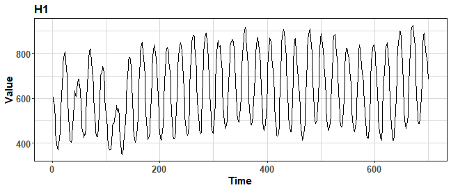

Bootstrap aggregating (bagging) is an ensemble meta-algorithm (introduced by Breiman in 1996), which creates multiple versions of learning set to produce multiple numbers of predictions. These predictions are then aggregated, for example by arithmetic mean. For time dependent data with a combination of statistical forecasting methods, the classical bagging can’t be used - so sampling (bootstrapping) with replacement. We have to sample data more sophisticated - based on seasonality or something similar. One of the used bootstrapping method is Moving Block Bootstrap (MBB) that uses a block (defined by seasonality for example) for creating new series. However, we don’t use the whole time series as it is, but we bootstrap only its remainder part from STL decomposition (this bootstrapping method was proposed by Bergmeir et al. in 2016).

This method is implemented in the forecast package in bld.mbb.bootstrap function, let’s use it on one time series from M4 competition dataset:

period <- 24*7 # weekly period
data_ts <- as.numeric(hourly_M4[[1]]$x)
data_boot_mbb <- bld.mbb.bootstrap(ts(data_ts, freq = period), 100)
data_plot <- data.table(Value = unlist(data_boot_mbb),
                        ID = rep(1:length(data_boot_mbb), each = length(data_ts)),
                        Time = rep(1:length(data_ts), length(data_boot_mbb))
                        )
 
ggplot(data_plot) +
  geom_line(aes(Time, Value, group = ID), alpha = 0.5) +
  geom_line(data = data_plot[.(1), on = .(ID)], aes(Time, Value),
            color = "firebrick1", alpha = 0.9, size = 0.8) +
  theme_ts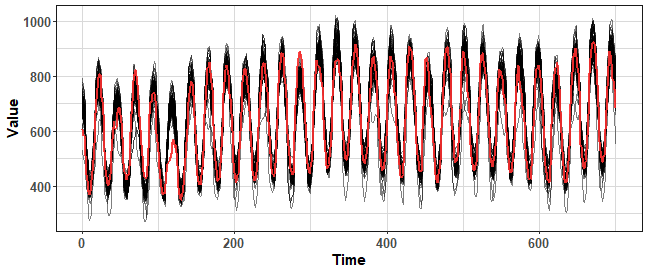

We can see that where values of the time series are low, there bld.mbb method fails to bootstrap new values around original ones (red line). Notice also that variance of bootstrapped time series is very high and values fly somewhere more than 30% against original values.

For this reason, I proposed a smoothed version of the bld.mbb method for reducing variance (Laurinec et al. 2019). I smoothed the remainder part from STL decomposition by exponential smoothing, so extreme noise was removed. Let’s use it (source code is available on my GitHub repo):

data_boot_smbb <- smo.bootstrap(ts(data_ts, freq = period), 100)
data_plot <- data.table(Value = unlist(data_boot_smbb),
                        ID = rep(1:length(data_boot_smbb), each = length(data_ts)),
                        Time = rep(1:length(data_ts), length(data_boot_smbb))
                        )
 
ggplot(data_plot) +
  geom_line(aes(Time, Value, group = ID), alpha = 0.5) +
  geom_line(data = data_plot[.(1), on = .(ID)], aes(Time, Value),
            color = "firebrick1", alpha = 0.9, size = 0.8) +
  theme_ts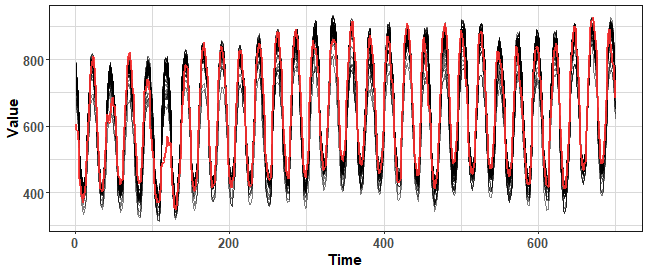

We can see that the variance was nicely lowered, but the final time series are sometimes really different from the original. It is not good when we want to use them for forecasting.

Therefore, I developed (designed) another two bootstrapping methods based on K-means clustering. The first step of the two methods is identical - automatic clustering of univariate time series - where automatic means that it estimates the number of clusters from a defined range of clusters by Davies-Bouldin index.

The first method, after clustering, samples new values from cluster members, so it isn’t creating new values. Let’s plot results:

data_boot_km <- KMboot(ts(data_ts, freq = period), 100, k_range = c(8, 10))
data_plot <- data.table(Value = unlist(data_boot_km),
                        ID = rep(1:length(data_boot_km), each = length(data_ts)),
                        Time = rep(1:length(data_ts), length(data_boot_km))
                       )
 
ggplot(data_plot) +
  geom_line(aes(Time, Value, group = ID), alpha = 0.5) +
  geom_line(data = data_plot[.(1), on = .(ID)], aes(Time, Value),
            color = "firebrick1", alpha = 0.9, size = 0.8) +
  theme_ts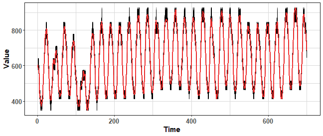

We can change the range of the number of clusters to be selected to lower to increase the variance of bootstrapped time series. Let’s try increase number of clusters to decrease variance:

data_boot_km <- KMboot(ts(data_ts, freq = period), 100, k_range = c(14, 20))
data_plot <- data.table(Value = unlist(data_boot_km),
                        ID = rep(1:length(data_boot_km), each = length(data_ts)),
                        Time = rep(1:length(data_ts), length(data_boot_km))
                        )
 
ggplot(data_plot) +
  geom_line(aes(Time, Value, group = ID), alpha = 0.5) +
  geom_line(data = data_plot[.(1), on = .(ID)], aes(Time, Value),
            color = "firebrick1", alpha = 0.9, size = 0.8) +
  theme_ts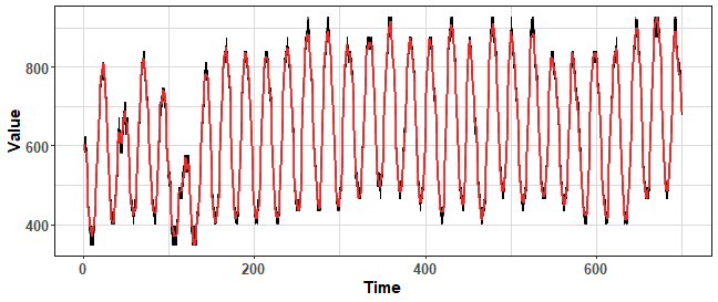

We can see that the variance is much lower against MBB based methods. But we have still the power to increase it if we change the range of number of clusters.

The second proposed K-means based method is sampling new values randomly from Gaussian distribution based on parameters of created clusters (mean and variance). Let’s use it on our selected time series:

data_boot_km.norm <- KMboot.norm(ts(data_ts, freq = period), 100, k_range = c(12, 20))
data_plot <- data.table(Value = unlist(data_boot_km.norm),
                        ID = rep(1:length(data_boot_km.norm), each = length(data_ts)),
                        Time = rep(1:length(data_ts), length(data_boot_km.norm))
)
 
ggplot(data_plot) +
  geom_line(aes(Time, Value, group = ID), alpha = 0.5) +
  geom_line(data = data_plot[.(1), on = .(ID)], aes(Time, Value),
            color = "firebrick1", alpha = 0.9, size = 0.8) +
  theme_ts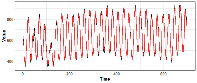

We can see nicely distributed values around the original time series, but will be it beneficial for forecasting?

We can also check all four bootstrapping methods in one plot by wrapper around above calls:

print_boot_series <- function(data, ntimes = 100, k_range = c(12, 20)) {
  
  data_boot_1 <- bld.mbb.bootstrap(data, ntimes)
  data_boot_2 <- smo.bootstrap(data, ntimes)
  data_boot_3 <- KMboot(data, ntimes, k_range = k_range)
  data_boot_4 <- KMboot.norm(data, ntimes, k_range = k_range)
  
  datas_all <- data.table(Value = c(unlist(data_boot_1), unlist(data_boot_2),
                                    unlist(data_boot_3), unlist(data_boot_4)),
                          ID = rep(rep(1:ntimes, each = length(data)), 4),
                          Time = rep(rep(1:length(data), ntimes), 4),
                          Method = factor(rep(c("MBB", "S.MBB", "KM", "KM.boot"),
                                              each = ntimes*length(data)))
  )
  
  datas_all[, Method := factor(Method, levels(Method)[c(3,4,1,2)])]
  
  print(ggplot(datas_all) +
          facet_wrap(~Method, ncol = 2) +
          geom_line(aes(Time, Value, group = ID), alpha = 0.5) +
          geom_line(data = datas_all[.(1), on = .(ID)], aes(Time, Value),
                    color = "firebrick1", alpha = 0.9, size = 0.8) +
          theme_ts)
 
}
 
print_boot_series(ts(hourly_M4[[200]]$x, freq = period))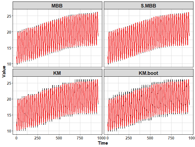

When the time series is non-stationary, the clustering bootstrapping methods can oscillate little-bit badly. The clustering-based bootstrapping methods could be enhanced by for example differencing to be competitive (applicable) for non-stationary time series with a strong linear trend.

Forecasting with bootstrapping

For evaluating four presented bootstrapping methods for time series, to see which is the most competitive in general, experiments with 6 statistical forecasting methods were performed on all 414 hourly time series from the M4 competition dataset. Forecasts from bootstrapped time series were aggregated by the median. Also, simple base methods were evaluated alongside seasonal naive forecast. The six chosen statistical base forecasting methods were:

• STL+ARIMA,
• STL+ETS (both forecast package),
• triple exponential smoothing with damped trend (smooth package - named ES (AAdA)),
• Holt-Winters exponential smoothing (stats package),
• dynamic optimized theta model (forecTheta package - named DOTM),
• and standard theta model (forecast package).

Forecasting results were evaluated by sMAPE and ranks sorted by sMAPE forecasting accuracy measure.

The source code that generates forecasts from the all mentioned methods above and process results are available on my GitHub repository.

The first visualization of results shows mean sMAPE by base forecasting method:

ggplot(res_all[, .(sMAPE = mean(sMAPE, na.rm = TRUE)), by = .(Base_method, Boot_method)]) +
  facet_wrap(~Base_method, ncol = 3, scales = "fix") +
  geom_bar(aes(Boot_method, sMAPE, fill = Boot_method, color = Boot_method), alpha = 0.8, stat = "identity") +
  geom_text(aes(Boot_method, y = sMAPE + 1, label = paste(round(sMAPE, 2)))) +
  scale_fill_d3() +
  scale_color_d3() +
  theme_ts +
  theme(axis.text.x = element_text(angle = 60, hjust = 1))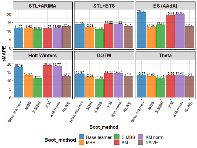

Best methods based on average sMAPE are STL+ETS with s.MBB and DOTM with s.MBB bootstrapping. Our proposed s.MBB bootstrapping method won’s 5 times from 6 based on average sMAPE.

The next graph shows boxplot of Ranks:

ggplot(res_all) +
  facet_wrap(~Base_method, ncol = 3, scales = "fix") +
  geom_boxplot(aes(Boot_method, Rank, fill = Boot_method), alpha = 0.8) +
  scale_fill_d3() +
  theme_ts +
  theme(axis.text.x = element_text(angle = 60, hjust = 1))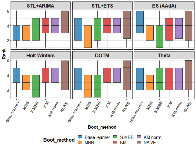

We can see very tight results amongst base learners, MBB and s.MBB methods.

So, let’s see average Rank instead:

ggplot(res_all[, .(Rank = mean(Rank, na.rm = TRUE)), by = .(Base_method, Boot_method)]) +
  facet_wrap(~Base_method, ncol = 3, scales = "fix") +
  geom_bar(aes(Boot_method, Rank, fill = Boot_method, color = Boot_method), alpha = 0.8,
           stat = "identity") +
  geom_text(aes(Boot_method, y = Rank + 0.22, label = paste(round(Rank, 2))), size = 5) +
  scale_fill_d3() +
  scale_color_d3() +
  theme_ts +
  theme(axis.text.x = element_text(angle = 60, hjust = 1))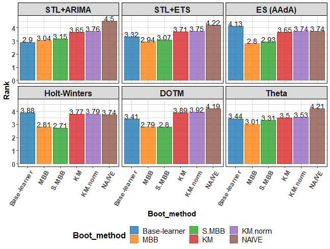

As was seen in the previous plot, it changes and it depends on a forecasting method, but very slightly better results have original MBB method over my s.MBB, but both beats base learner 5 times from 6. KM-based bootstraps failed to beat base learner 4 times from 6.

Let’s be more curious about distribution of Ranks…I will show you plot of Rank counts:

ggplot(res_all[, .(N = .N), by = .(Base_method, Boot_method, Rank)]
       [, Rank := factor(Rank)],
       aes(Boot_method, N)) +
  facet_wrap(~Base_method, ncol = 3, scales = "free") +
  geom_bar(aes(fill = Rank,
               color = Rank),
           alpha = 0.75, position = "dodge", stat = "identity") +
  scale_fill_d3() +
  scale_color_d3() +
  theme_ts +
  theme(axis.text.x = element_text(size = 10, angle = 60, hjust = 1))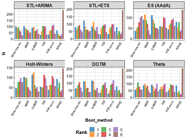

We can see that KM-based bootstrapping can be first or second too! Around 25-times for each forecasting method were these 2 boot. methods first, and around 2-times more second…not that bad. Also, the seasonal naive forecast can be on some types of time series best against more sophisticated statistical forecasting methods… However, MBB and s.MBB methods are best and most of the time are in the first two ranks.

Conclusion

In this blog post, I showed you how to simply use four various bootstrapping methods on time series data. Then, the results of experiments performed on the M4 competition dataset were shown. Results suggest that bootstrapping can be very useful for improving forecasting accuracy.

References

[1] Bergmeir C., Hyndman R.J., Benitez J.M.: Bagging exponential smoothing methods using stl decomposition and box-cox transformation. International Journal of Forecasting, 32(2):303-312, (2016)

[2] Laurinec P., Loderer M., Lucka M. et al.: Density-based unsupervised ensemble learning methods for time series forecasting of aggregated or clustered electricity consumption, Journal Intelligent Information Systems, 53(2):219-239, (2019). DOI link