Dangerous streets of Bratislava! Animated maps using open data in R
At the work recently, I wanted to make some interesting start-up pitch (presentation) ready animated visualization and got some first experience with spatial data (e.g. polygons). I enjoyed working with such a type of data and I wanted to improve on working with them, so I decided to try to visualize something interesting with Bratislava (Slovakia) open-data and OpenStreetMaps. I ended with animated maps of violations on Bratislava streets through the time of 2 and a half years.
Since spatial time series are analyzed in this post, it still sticks with the blog domain and it is time series data mining :) You can read more about time series forecasting, representations and clustering in my previous blog posts here.
Aaand teaser, what I will create in this blog post:
In this blog post you will learn how to:
- get free city district polygons data from OpenStreetMaps API,
- get free street lines (polygons) coordinates from OpenStreetMaps API,
- visualize polygons and street lines with
ggplot2andggmap, - merge spatial data with violation data represented as time series,
- animate spatial data combined with violation time series with
gganimate.
Bratislava Open-Data
The ultimate goal is to show where and when are the most dangerous places in the capital of Slovakia - Bratislava. For this task, I will use open-data that cover violations gathered from the city police with locations (city district and street name) and time-stamp.
Firstly, load all the needed packages.
library(data.table) # handling data
library(lubridate) # handling timestamps
library(stringi) # text processing
library(osmdata) # OSM data API
# library(nominatim) # alternative OSM data API
library(sf) # handling spatial data
library(ggplot2) # visualisations
library(ggsci) # color pallets
library(ggmap) # map vis
library(gganimate) # animations
library(magick) # image handling
Then, let’s download the violations data from opendata.bratislava.sk webpage and translate Slovak column names to English.
data_violation_17 <- fread("https://opendata.bratislava.sk/dataset/download/pocet-priestupkov-podla-druhu-udalosti-v-roku-r/1",
                           encoding = "Latin-1")
data_violation_18 <- fread("https://opendata.bratislava.sk/dataset/download/pocet-priestupkov-podla-druhu-udalosti-v-roku-/1",
                           encoding = "Latin-1")
data_violation_19 <- fread("https://opendata.bratislava.sk/dataset/download/pocet-priestupkov-podla-druhu-udalosti-----ethyanzgrthar/1",
                           encoding = "Latin-1")

# colnames to English
setnames(data_violation_17, colnames(data_violation_17), c("Date_Time", "Group_vio",
                                                           "Type_vio", "Street", "Place"))
setnames(data_violation_18, colnames(data_violation_18), c("Date_Time", "Group_vio",
                                                           "Type_vio", "Street", "Place"))
setnames(data_violation_19, colnames(data_violation_19), c("Date_Time", "Group_vio",
                                                           "Type_vio", "Street", "Place"))
Let’s bind all the data together.
data_violation <- rbindlist(list(data_violation_17, data_violation_18, data_violation_19),
                            use.names = T)
Next, I will transform Date_Time to POCIXct format and generate time aggregation features - Year and Month - Year_M.
data_violation[, Date_Time := dmy_hm(Date_Time)]
data_violation[, Date := date(Date_Time)]

# Aggregation features
data_violation[, Month := month(Date_Time)]
data_violation[, Year := year(Date_Time)]
data_violation[, Year_M := Year + Month/100]
Let’s see how many violations have each Place (city district) for whole available period (2017-2019.09):
data_violation[, .N, by = .(Place)]## Place N
## 1: Stare Mesto 68714
## 2: Karlova Ves 11462
## 3: Petrzalka 17062
## 4: Dubravka 6307
## 5: Ruzinov 21352
## 6: Vajnory 1194
## 7: Pod. Biskupice 1590
## 8: Vrakuna 1262
## 9: Nove Mesto 17964
## 10: Devin 269
## 11: Raca 2390
## 12: Devinska Nova Ves 1406
## 13: Lamac 1455
## 14: Jarovce 66
## 15: Zah. Bystrica 928
## 16: Rusovce 753
## 17: Cunovo 569We can see that Old-town (Stare Mesto) rocks in this statistic..obviously - e.g. lot of tourists. There are also some misunderstand Slavic letters. We should get rid of them - in the blog post there we be lot of handling of these special Slavic (Slovak) symbols.
data_violation[, Place := stri_trans_general(Place, "Latin-ASCII")]
data_violation[.("Eunovo"), on = .(Place), Place := "Cunovo"]
data_violation[.("Raea"), on = .(Place), Place := "Raca"]
data_violation[.("Vrakuoa"), on = .(Place), Place := "Vrakuna"]
data_violation[.("Lamae"), on = .(Place), Place := "Lamac"]
I will extract only types of violations that relate to the bad behavior of people, like harassment, using alcoholic beverages on public space and related things. So, I will not extract traffic violations like bad car parking, etc. For this task, I need to extract codes of violations:
data_violation[, Group_vio_ID := as.numeric(substr(Group_vio, 1, 4))]
# our codes are: 4836, 5000, 4834, 4700, 4838, 4828, 4839,
# 4813, 9803, 4840, 4841, 9809, 3000, 9806, 4900
Polygons of city districts
I want to show a number of crimes per city district and street (so both place information) on a map, so I need to get coordinates of city districts and streets. Let’s get polygons of city districts first using OpenStreetMap API.
poly_sm <- getbb(place_name = "Stare Mesto Bratislava", format_out = "polygon")
poly_nm <- getbb(place_name = "Nove Mesto Bratislava", format_out = "polygon")
poly_ruz <- getbb(place_name = "Ruzinov Bratislava", format_out = "polygon")
poly_raca <- getbb(place_name = "Raca Bratislava", format_out = "polygon")
poly_petr <- getbb(place_name = "Petrzalka Bratislava", format_out = "polygon")
poly_kv <- getbb(place_name = "Karlova Ves Bratislava", format_out = "polygon")
poly_dubr <- getbb(place_name = "Dubravka Bratislava", format_out = "polygon")
poly_vajn <- getbb(place_name = "Vajnory Bratislava", format_out = "polygon")
poly_lamac <- getbb(place_name = "Lamac Bratislava", format_out = "polygon")
poly_vrak <- getbb(place_name = "Vrakuna Bratislava", format_out = "polygon")
poly_pd <- getbb(place_name = "Podunajske Biskupice Bratislava", format_out = "polygon")
poly_jar <- getbb(place_name = "Jarovce Bratislava", format_out = "polygon")
poly_dnv <- getbb(place_name = "Devinska Nova Ves Bratislava", format_out = "polygon")
poly_rus <- getbb(place_name = "Rusovce Bratislava", format_out = "polygon")
poly_zb <- getbb(place_name = "Zahorska Bystrica Bratislava", format_out = "polygon")
poly_devin <- getbb(place_name = "Devin Bratislava", format_out = "polygon")
poly_cun <- getbb(place_name = "Cunovo Bratislava", format_out = "polygon")
Let’s bind all the districts data of Bratislava.
data_poly_ba <- rbindlist(list(
  as.data.table(poly_sm)[, Place := "Stare Mesto"],
  as.data.table(poly_nm[[1]])[, Place := "Nove Mesto"],
  as.data.table(poly_ruz[[1]])[, Place := "Ruzinov"],
  as.data.table(poly_raca)[, Place := "Raca"],
  as.data.table(poly_petr)[, Place := "Petrzalka"],
  as.data.table(poly_kv[[1]])[, Place := "Karlova Ves"],
  as.data.table(poly_dubr[[1]])[, Place := "Dubravka"],
  as.data.table(poly_vajn[[1]])[, Place := "Vajnory"],
  as.data.table(poly_lamac[[1]])[, Place := "Lamac"],
  as.data.table(poly_vrak[[1]])[, Place := "Vrakuna"],
  as.data.table(poly_pd[[1]])[, Place := "Pod. Biskupice"],
  as.data.table(poly_jar[[1]])[, Place := "Jarovce"],
  as.data.table(poly_dnv[[1]])[, Place := "Devinska Nova Ves"],
  as.data.table(poly_rus[[1]])[, Place := "Rusovce"],
  as.data.table(poly_zb[[1]])[, Place := "Zah. Bystrica"],
  as.data.table(poly_devin[[1]])[, Place := "Devin"],
  as.data.table(poly_cun[[1]])[, Place := "Cunovo"]
))

setnames(data_poly_ba, c("V1", "V2"), c("lon", "lat"))
data_poly_ba[, Place := factor(Place)]
Let’s visualize simply the districts.
ggplot(data_poly_ba) +
  geom_polygon(aes(x = lon, y = lat,
                   fill = Place, color = Place)) +

  theme_void()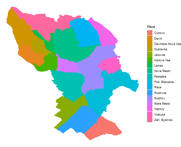
For animation and visualization purposes, I need to aggregate violations data by districts (Place) and Year+Month columns (Year_M).
data_violation_agg_place <- copy(data_violation[.(c(4836, 5000, 4834, 4700, 4838,
                                                    4828, 4839, 4813, 9803, 4840,
                                                    4841, 9809, 3000, 9806, 4900)),
                                                on = .(Group_vio_ID),
                                                .(N = .N),
                                                by = .(Place, Year_M)])
The next step is to merge polygon data with aggregated violation data:
data_places <- merge(data_poly_ba[, .(Place, lon, lat)],
                     data_violation_agg_place[, .(Place, N_violation = N, Year_M)],
                     by = "Place",
                     all.y = T,
                     allow.cartesian = T)
Let’s also compute mean coordinates for every district for showing theirs names on a graph.
data_poly_ba_mean_place <- copy(data_poly_ba[, .(lon = mean(lon),
                                                 lat = mean(lat)),
                                             by = .(Place)])
Let’s test visualization of violations on June 2019:
ggplot() +
  geom_polygon(data = data_places[.(2019.06), on = .(Year_M)],
               aes(x = lon, y = lat,
                   fill = N_violation,
                   group = Place),
               color = "grey40") +
  scale_fill_material("grey") +
  geom_label(data = data_poly_ba_mean_place,
             aes(x = lon, y = lat, label = Place),
             color = "black", fill = "dodgerblue1", alpha = 0.65) +
  theme_void()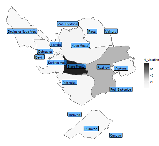
Street lines coordinates
The next step is to download street coordinates from OpenStreetMaps.
Firstly, we have to extract unique street names from violation data, and handle Slovak letters and other punctuation for easier matching by street name.
dt_uni_streets <- copy(data_violation[, .(Place = data.table::first(Place)),
by = .(Street)])
dt_uni_streets[, Street_edit := gsub(pattern = "È", replacement = "C", x = Street)]
dt_uni_streets[, Street_edit := gsub(pattern = "ò", replacement = "n", x = Street_edit)]
dt_uni_streets[, Street_edit := gsub(pattern = "è", replacement = "c", x = Street_edit)]
dt_uni_streets[, Street_edit := gsub(pattern = "\u009d", replacement = "t", x = Street_edit)]
dt_uni_streets[, Street_edit := gsub(pattern = "¾", replacement = "l", x = Street_edit)]
dt_uni_streets[, Street_edit := gsub(pattern = "¼", replacement = "L", x = Street_edit)]
dt_uni_streets[, Street_edit := gsub(pattern = "ò", replacement = "n", x = Street_edit)]
dt_uni_streets[, Street_edit := gsub(pattern = "_", replacement = "", x = Street_edit)]
dt_uni_streets[, Street_edit := gsub(pattern = "ï", replacement = "d", x = Street_edit)]
dt_uni_streets[, Street_edit := gsub(pattern = "Ã ", replacement = "r", x = Street_edit)]
dt_uni_streets[, Street_edit := stri_trans_general(Street_edit, "Latin-ASCII")]
dt_uni_streets[, Street_edit := sub(" - MC.*", "", Street_edit)]
dt_uni_streets[, Street_edit := gsub(pattern = "Nam.", replacement = "Namestie ",
x = Street_edit)]
dt_uni_streets[, Street_query := gsub(pattern = " ", replacement = "+", x = Street_edit)]
dt_uni_streets[, Street_query := paste0(Street_query, "+Bratislava")]Let’s get all streets coordinates of Bratislava just by one (powerful) command, again using OSM API:
ba_bb <- getbb(place_name = "Bratislava")

bratislava <- opq(bbox = ba_bb) %>%
  add_osm_feature(key = 'highway') %>%
  osmdata_sf() %>%
  osm_poly2line()
Let’s plot it:
ggplot(data = bratislava$osm_lines) +
  geom_sf() +
  theme_bw()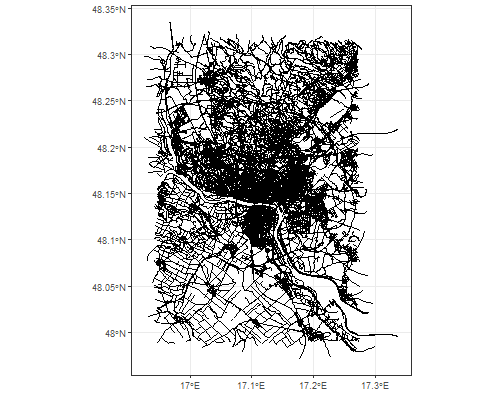
Pretty nice web.
Now, we need to handle again street names downloaded from OSM. I will extract only available streets from violation data:
street_names <- data.table(Street = unique(bratislava$osm_lines$name))

street_names[, Street_edit := gsub(pattern = "Ã", replacement = "i", x = Street)]
street_names[, Street_edit := gsub(pattern = "i©", replacement = "e", x = Street_edit)]
street_names[, Street_edit := gsub(pattern = "i¡", replacement = "a", x = Street_edit)]
street_names[, Street_edit := gsub(pattern = "iº", replacement = "u", x = Street_edit)]
street_names[, Street_edit := gsub(pattern = "ž", replacement = "z", x = Street_edit)]
street_names[, Street_edit := gsub(pattern = "ľ", replacement = "l", x = Street_edit)]
street_names[, Street_edit := gsub(pattern = "Ä\u008d", replacement = "c", x = Street_edit)]
street_names[, Street_edit := gsub(pattern = "Å¡", replacement = "s", x = Street_edit)]
street_names[, Street_edit := gsub(pattern = "Ľ", replacement = "L", x = Street_edit)]
street_names[, Street_edit := gsub(pattern = "ň", replacement = "n", x = Street_edit)]
street_names[, Street_edit := gsub(pattern = "i½", replacement = "y", x = Street_edit)]
street_names[, Street_edit := gsub(pattern = "Å•", replacement = "r", x = Street_edit)]
street_names[, Street_edit := gsub(pattern = "i³", replacement = "o", x = Street_edit)]
street_names[, Street_edit := gsub(pattern = "i¤", replacement = "a", x = Street_edit)]
street_names[, Street_edit := gsub(pattern = "Ž", replacement = "Z", x = Street_edit)]
street_names[, Street_edit := gsub(pattern = "Ã… ", replacement = "S", x = Street_edit)]
street_names[, Street_edit := gsub(pattern = "Ã…Â¥", replacement = "t", x = Street_edit)]
street_names[, Street_edit := gsub(pattern = "Č", replacement = "C", x = Street_edit)]
street_names[, Street_edit := gsub(pattern = "Ä\u008f", replacement = "d", x = Street_edit)]
street_names[, Street_edit := gsub(pattern = "i¶", replacement = "o", x = Street_edit)]
street_names[, Street_edit := gsub(pattern = "Å‘", replacement = "o", x = Street_edit)]
street_names[, Street_edit := gsub(pattern = "Ä›", replacement = "e", x = Street_edit)]
street_names[, Street_edit := gsub(pattern = "Ä›", replacement = "e", x = Street_edit)]

street_names[, Street_edit := stri_trans_general(Street_edit, "Latin-ASCII")]
street_names[, Street_edit := gsub(pattern = "i-", replacement = "i", x = Street_edit)]
street_names[, Street_edit := gsub(pattern = "A ", replacement = "S", x = Street_edit)]

street_names[dt_uni_streets, on = .(Street_edit)]
street_names_vio <- copy(street_names[dt_uni_streets, on = .(Street_edit),
                                      Street_orig := i.Street])[!is.na(Street_orig)]
We lost some street data from the dataset by not exact matched street names.
Let’s subset the street data.
ba_streets_vio <- bratislava$osm_lines
ba_streets_vio <- ba_streets_vio[ba_streets_vio$name %in% street_names_vio$Street,]
ba_streets_vio <- ba_streets_vio[!is.na(ba_streets_vio$name),]
Now, I will transform data to standard lon/lat matrix (data.table class) format instead of sf object (I highly recommend this for next ggplot usage).
data_streets_st <- data.table::data.table(sf::st_coordinates(ba_streets_vio$geometry))Next, I will bound streets by existing polygons of Bratislava and add merging column - Street_edit:
ba_streets_vio$L1 <- 1:nrow(ba_streets_vio)
data_streets_st <- merge(data_streets_st, as.data.table(ba_streets_vio)[, .(L1, name)],
                         by = "L1")
data_streets_st[street_names_vio[, .(name, Street_edit)], on = .(name),
                Street_edit := i.Street_edit]
setnames(data_streets_st, c("X", "Y"), c("lon", "lat"))
data_streets_st <- data_streets_st[!lon > data_poly_ba[, max(lon)]]
data_streets_st <- data_streets_st[!lon < data_poly_ba[, min(lon)]]
data_streets_st <- data_streets_st[!lat > data_poly_ba[, max(lat)]]
Let’s also aggregate violation data by street names and Year + Month (Year_M):
data_violation_agg_street <- copy(data_violation[.(c(4836, 5000, 4834, 4700, 4838,
                                                    4828, 4839, 4813, 9803, 4840,
                                                    4841, 9809, 3000, 9806, 4900)),
                                                 on = .(Group_vio_ID),
                                                 .(N = .N), by = .(Street, Year_M)])

setorder(data_violation_agg_street, Year_M, -N)
Let’s add look-up column Street_edit to aggregated data and merge spatial street data with violation data.
data_violation_agg_street[dt_uni_streets, on = .(Street), Street_edit := i.Street_edit]

data_streets_st <- merge(data_streets_st,
                         data_violation_agg_street[, .(Street_edit, N_violations = N, Year_M)],
                         by = "Street_edit",
                         all.y = T,
                         allow.cartesian = TRUE)
Now, I will transform integers of the number of violations to reasonable factors segments:
data_streets_st[N_violations >= 11, N_violation_type := "> 11"]
data_streets_st[N_violations >= 6 & N_violations < 11, N_violation_type := "(6, 10)"]
data_streets_st[N_violations >= 3 & N_violations < 6, N_violation_type := "(3, 5)"]
data_streets_st[N_violations <= 2, N_violation_type := "< 2"]
data_streets_st[, N_violations_per_street := factor(N_violation_type,
                                                    levels = c("< 2",  "(3, 5)",
"(6, 10)", "> 11"))]levels(data_streets_st$N_violations_per_street)## [1] "< 2" "(3, 5)" "(6, 10)" "> 11"Let’s see what we extracted so far for streets in one example year-month…
ggplot(data_streets_st[!is.na(L1)][.(2019.06),
                                   on = .(Year_M)]) +
  geom_line(aes(lon, lat, group = L1,
                color = N_violations_per_street),
            size = 1.4) +
  scale_color_brewer(palette = "Reds") +
  theme_bw()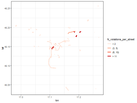
ggmap
Since, we will use ggmap for visualizations, we need to extract map image of Bratislava:
bbox <- make_bbox(lon, lat, data = data_poly_ba, f = .01) # used our polygons
map_ba <- get_map(location = bbox, source = 'stamen', maptype = "watercolor")
Now, let’s make it altogether to one visualization - so violations by city districts and also streets for one time-stamp (Year_M).
ggmap(map_ba, extent = "device") +
  geom_polygon(data = data_places[.(2019.06),
                                  on = .(Year_M)],
               aes(x = lon, y = lat,
                   fill = N_violation,
                   group = Place),
               color = "grey40") +
  scale_fill_material("grey", alpha = 0.75) +
  geom_line(data = data_streets_st[!is.na(L1)][.(2019.06),
                                               on = .(Year_M)],
            aes(lon, lat, group = L1, color = N_violations_per_street),
            size = 1.4) +
  scale_color_brewer(palette = "Reds") +
  geom_label(data = data_poly_ba_mean_place,
             aes(x = lon, y = lat, label = Place,
                 fill = NA_real_),
             color = "black", fill = "dodgerblue1", alpha = 0.75) +
  labs(fill = "N_vio_district", color = "N_vio_street") +
  guides(color = guide_legend(override.aes = list(size = 2))) +
  theme_void()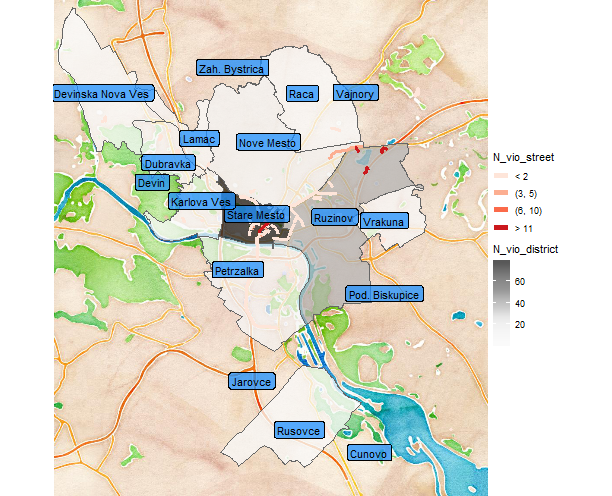
I will also extract the most violated streets by Year+Month for labeling purposes.
data_streets_st_max <- copy(data_streets_st[!is.na(L1),
                                            .SD[N_violations == max(N_violations, na.rm = T)],
                                            by = .(Year_M)])

data_streets_st_max[, unique(Street_edit)] # the unique month "winners"
data_streets_st_max <- copy(data_streets_st_max[, .(lon = mean(lon),
                                                    lat = mean(lat),
                                                    Street_edit = first(Street_edit),
                                                    N_violations = first(N_violations),
                                                    N_violations_per_street =
                                                      first(N_violations_per_street)
                                                    ),
                                                by = .(Year_M)])
As we noticed so far, the most violated city district is Old-town, so I will create also zoomed visualization for this city district like this (using coord_map function):
ggmap(map_ba) +
  geom_polygon(data = data_places[.(2019.06), on = .(Year_M)],
               aes(x = lon, y = lat,
                   fill = N_violation,
                   group = Place
               ),
               color = "grey40") +
  scale_fill_material("grey", alpha = 0.75) +
  geom_line(data = data_streets_st[!is.na(L1)][.(2019.06), on = .(Year_M)],
            aes(lon, lat, group = L1, color = N_violations_per_street),
            size = 1.4) +
  geom_label(data = data_streets_st_max[.(2019.06), on = .(Year_M)],
             aes(x = lon, y = lat,
                 label = paste0(Street_edit, " - ", N_violations)
             ),
             color = "black",
             fill = "firebrick2",
             size = 4.5,
             alpha = 0.75
  ) +
  scale_color_brewer(palette = "Reds") +
  geom_label(data = data_poly_ba_mean_place,
             aes(x = lon, y = lat, label = Place,
                 fill = NA_real_),
             color = "black", fill = "dodgerblue1",
             alpha = 0.75, size = 4.5) +
  coord_map(
    xlim=c(data_poly_ba[.("Stare Mesto"), on = .(Place), min(lon)],
           data_poly_ba[.("Stare Mesto"), on = .(Place), max(lon)]),
    ylim= c(data_poly_ba[.("Stare Mesto"), on = .(Place), min(lat)],
            data_poly_ba[.("Stare Mesto"), on = .(Place), max(lat)])
  ) +
  labs(fill = "N_vio_district", color = "N_vio_street") +
  guides(color = guide_legend(ncol = 1, override.aes = list(size = 2),
                              title.position = "top"),
         fill = guide_legend(nrow = 2, title.position = "top")) +
  theme_bw() +
  theme(axis.text = element_blank(),
        axis.line = element_blank(),
        axis.title = element_blank(),
        axis.ticks = element_blank(),
        legend.text = element_text(size = 13),
        legend.title = element_text(size = 14, face = "bold"),
        legend.background = element_rect(fill = "white"),
        legend.key = element_rect(fill = "white"),
        legend.position = "bottom")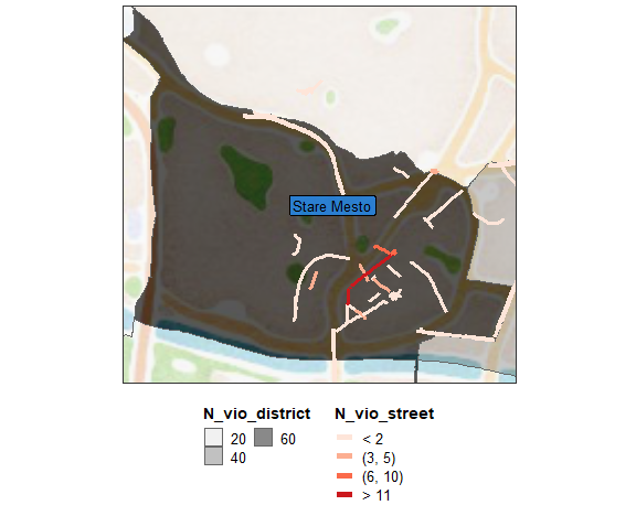
Using ggnanimate
We have all prepared to create some interesting animated map.
For this purpose, I will use the gganimate package that simply uses the transition_states function that combines our previously prepared ggplot2 and ggmap plot and time feature Year_M.
Let’s firstly animate the whole city picture.
gg_ba_anim_lines <- ggmap(map_ba, extent = "device") +
  geom_polygon(data = data_places,
               aes(x = lon, y = lat,
                   fill = N_violation,
                   group = Place),
               color = "grey40") +
  scale_fill_material("grey", alpha = 0.7) +
  geom_line(data = data_streets_st[!is.na(L1)],
            aes(lon, lat,
                group = L1,
                color = N_violations_per_street
            ),
            size = 1.4
  ) +
  scale_color_brewer(palette = "Reds") +
  labs(fill = "N_vio_district", color = "N_vio_street") +
  geom_label(data = data_poly_ba_mean_place,
             aes(x = lon, y = lat, label = Place,
                 fill = NA_real_),
             color = "black", fill = "dodgerblue1",
             alpha = 0.75, size = 4.5) +
  transition_states(reorder(Year_M, Year_M), transition_length = 2,
                    state_length = 1) +
  labs(title = "Year.Month - {closest_state}") +
  guides(color = FALSE, fill = FALSE) +
  theme_void() +
  theme(plot.title = element_text(size = 16, face = "bold")
  )

# save animation to object
anim_whole <- animate(gg_ba_anim_lines, duration = 46, width = 700, height = 750)
Then, let’s animate zoomed map of Old-town district.
gg_ba_anim_lines_zoom <- ggmap(map_ba, extent = "device") +
  geom_polygon(data = data_places,
               aes(x = lon, y = lat,
                   fill = N_violation,
                   group = Place),
               color = "grey40") +
  scale_fill_material("grey", alpha = 0.7) +
  geom_line(data = data_streets_st[!is.na(L1)],
            aes(lon, lat,
                group = L1,
                color = N_violations_per_street
            ),
            size = 1.4
  ) +
  scale_color_brewer(palette = "Reds") +
  geom_label(data = data_streets_st_max,
             aes(x = lon, y = lat,
                 label = paste0(Street_edit, " - ", N_violations)
             ),
             color = "black", fill = "firebrick2",
             alpha = 0.75, size = 4.5
  ) +
  geom_label(data = data_poly_ba_mean_place,
             aes(x = lon, y = lat, label = Place,
                 fill = NA_real_),
             color = "black", fill = "dodgerblue1",
             alpha = 0.75, size = 4.5
  ) +
  coord_map(
    xlim=c(data_poly_ba[.("Stare Mesto"), on = .(Place), min(lon)],
           data_poly_ba[.("Stare Mesto"), on = .(Place), max(lon)]),
    ylim= c(data_poly_ba[.("Stare Mesto"), on = .(Place), min(lat)],
            data_poly_ba[.("Stare Mesto"), on = .(Place), max(lat)])
  ) +
  transition_states(reorder(Year_M, Year_M), transition_length = 2,
                    state_length = 1) +
  labs(fill = "N_vio_district", color = "N_vio_street") +
  guides(color = guide_legend(ncol = 1, override.aes = list(size = 2),
                              title.position = "top"),
         fill = guide_legend(nrow = 2, title.position = "top")) +
  theme_bw() +
  theme(axis.text = element_blank(),
        axis.line = element_blank(),
        axis.title = element_blank(),
        axis.ticks = element_blank(),
        legend.text = element_text(size = 13),
        legend.title = element_text(size = 14, face = "bold"),
        legend.background = element_rect(fill = "white"),
        legend.key = element_rect(fill = "white"),
        legend.position = "bottom")

# save animation to object
anim_zoom <- animate(gg_ba_anim_lines_zoom, duration = 46, width = 700, height = 750)
GIFS binding with magick package
Now, we have to bind these two animations into one GIF. I will do it by functions from the magick package.
a_mgif <- image_read(anim_whole)
b_mgif <- image_read(anim_zoom)

new_gif <- image_append(c(a_mgif[1],
                          b_mgif[1]))

for(i in 2:100){
  combined <- image_append(c(a_mgif[i],
                             b_mgif[i]))
  new_gif <- c(new_gif, combined)
}

# final!
new_gif
Voilaaa:
For full resolution - right click on the gif and click on the view image option.
We can see that at the end of the observed period, so the summer of 2019, the Old-town district has even-more violations than usual. That can be caused by multiple factors…
Also notice, that peripheral areas of districts as Ruzinov and Vrakuna have streets with repeating multiple violations.
Streets with the most violations
Let’s see some of the most violated streets as time series as we seen in the animation.
times <- data.table(Year_M = data_violation_agg_street[, sort(unique(Year_M))])
times[, Date := as.Date("2017-01-01")]
times[, row_id := 1:.N]
times[, Date := Date + row_id*30.4]

data_vio_most_street <- copy(data_violation_agg_street[
  .(c("Michalska", "Postova",
      "Rybarska brana", "Namestie slobody")),
  on = .(Street_edit)])

data_vio_most_street[times, on = .(Year_M), Date := i.Date]
setnames(data_vio_most_street, "N", "N_violations")

ggplot(data_vio_most_street) +
  geom_line(aes(Date, N_violations, color = Street_edit), size = 0.8) +
  theme_bw()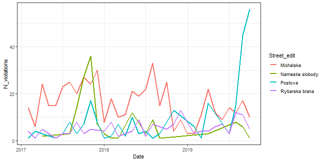
The most of the time, Michalska street in the historical center of the Old-town was the most violated street, but the last three months is Postova the “winner of the most violated street”…this is maybe because of the new city-police station nearby.
Summary
In this blog post, I showed you how to:
- work with different spatial data as polygons, street lines or map images,
- combine these spatial objects with external data as city violation time series,
- create animated maps using packages as
ggplot2,ggmap,gganimate, andmagick.
I hope, you will use these information with your spatial-time series data combo for creating some interesting visualization :)
The source code for this blog post can be found on my GitHub repository.
Seven coffees were consumed while writing this article.
If you’ve found it valuable, please consider supporting my work and...