Multivariate Regression Ensemble Models for Errors Prediction
In the last blog post about Multistep forecasting losses, I showed the usage of the fantastic method adam from the smooth R package on household electricity consumption data, and compared it with benchmarks.
Since I computed predictions from 10 methods/models for a long period of time, it would be nice to create some ensemble models for precise prediction for our household consumption data. For that purpose, it would be great to predict for example future errors of these methods. It is used in some known ensemble methods, which are not direct about stacking. Predicting errors can be beneficial for prediction weighting or for predicting the rank of methods (i.e. best one prediction). For the sake of learning something new, I will try multivariate regression models, so learning from multiple targets at once. At least, it has the benefit of simplicity, that we need only one model for all base prediction models.
What I will show you in this post:
- Prediction of forecasting errors (absolute residuals) of simple exponential smoothing methods.
- Usage of multivariate multiple linear regression benchmarks.
- Check of right rank prediction of forecasting methods.
- Catboost MultiRMSE capability and evaluation if it is more powerful than linear models.
- Computation of two types of ensemble predictions from predicted errors.
Simple forecasting methods error prediction
In the beginning, we need to load the required packages, be aware that catboost has to be installed by the devtools package in R.
library(data.table)
library(lubridate)
library(TSrepr)
library(ggplot2)
library(dygraphs)
library(glmnet)
# devtools::install_url('https://github.com/catboost/catboost/releases/download/v1.2.2/catboost-R-Windows-1.2.2.tgz')
library(catboost)
I will use predictions and errors from a previous blog post, you can download them from my GitHub repository.
load("_rmd/data_household_predictions.Rdata")
data_predictions_all
## Date_Time Load_real Load_predicted model
## 1: 2023-01-30 00:00:00 0.274 -0.7679345 STL+ETS
## 2: 2023-01-30 00:15:00 0.363 -0.7959601 STL+ETS
## 3: 2023-01-30 00:30:00 0.342 -0.7443988 STL+ETS
## 4: 2023-01-30 00:45:00 0.391 -0.8461708 STL+ETS
## 5: 2023-01-30 01:00:00 0.230 -0.8708582 STL+ETS
## ---
## 205436: 2023-08-31 22:45:00 0.080 0.4030999 ADAM-GPL
## 205437: 2023-08-31 23:00:00 0.039 0.2060178 ADAM-GPL
## 205438: 2023-08-31 23:15:00 0.087 0.2489654 ADAM-GPL
## 205439: 2023-08-31 23:30:00 0.080 0.1719251 ADAM-GPL
## 205440: 2023-08-31 23:45:00 0.040 0.4710469 ADAM-GPLWe will model absolute errors of predictions:
data_predictions_all[, Error := abs(Load_real - Load_predicted)]To be able to model all method’s predictions at once, we need to cast predictions and errors to wide form.
data_predictions_all_casted <- dcast(data_predictions_all,
                                     formula = Date_Time ~ model,
                                     value.var = c("Load_predicted", "Error"))

setnames(data_predictions_all_casted,
         colnames(data_predictions_all_casted),
         gsub("-", "_", colnames(data_predictions_all_casted)))
setnames(data_predictions_all_casted,
         colnames(data_predictions_all_casted),
         gsub("\\+", "_", colnames(data_predictions_all_casted)))

str(data_predictions_all_casted)
## Classes 'data.table' and 'data.frame': 20544 obs. of 21 variables:
## $ Date_Time : POSIXct, format: "2023-01-30 00:00:00" "2023-01-30 00:15:00" ...
## $ Load_predicted_ADAM_GPL : num 0.658 0.679 0.447 0.366 0.288 ...
## $ Load_predicted_ADAM_GTMSE: num 0.663 0.68 0.449 0.373 0.296 ...
## $ Load_predicted_ADAM_MAE : num 0.324 0.462 0.34 0.349 0.29 ...
## $ Load_predicted_ADAM_MAEh : num 0.545 0.566 0.334 0.253 0.175 ...
## $ Load_predicted_ADAM_MSCE : num 0.676 0.761 0.603 0.597 0.466 ...
## $ Load_predicted_ADAM_MSE : num 0.276 0.394 0.257 0.262 0.246 ...
## $ Load_predicted_ADAM_MSEh : num 0.662 0.681 0.452 0.377 0.299 ...
## $ Load_predicted_ADAM_TMSE : num 0.663 0.68 0.449 0.373 0.296 ...
## $ Load_predicted_STL_ARIMA : num -0.386 -0.412 -0.406 -0.482 -0.529 ...
## $ Load_predicted_STL_ETS : num -0.768 -0.796 -0.744 -0.846 -0.871 ...
## $ Error_ADAM_GPL : num 0.3839 0.316 0.1048 0.0248 0.0576 ...
## $ Error_ADAM_GTMSE : num 0.389 0.3168 0.1067 0.0183 0.0659 ...
## $ Error_ADAM_MAE : num 0.0504 0.09894 0.00155 0.04186 0.06019 ...
## $ Error_ADAM_MAEh : num 0.27104 0.20306 0.00819 0.1378 0.0554 ...
## $ Error_ADAM_MSCE : num 0.402 0.398 0.261 0.206 0.236 ...
## $ Error_ADAM_MSE : num 0.00248 0.03124 0.08472 0.12901 0.01597 ...
## $ Error_ADAM_MSEh : num 0.3884 0.3179 0.1097 0.0137 0.0692 ...
## $ Error_ADAM_TMSE : num 0.389 0.3168 0.1067 0.0183 0.0659 ...
## $ Error_STL_ARIMA : num 0.66 0.775 0.748 0.873 0.759 ...
## $ Error_STL_ETS : num 1.04 1.16 1.09 1.24 1.1 ...
## - attr(*, ".internal.selfref")=<externalptr>
## - attr(*, "sorted")= chr "Date_Time"Since we will train the regression model, there can be added also other helpful features. Let’s define helping daily and weekly seasonality features in the form of Sinus and Cosines. You can add also other features like holidays and weather parameters if it makes sense for your case.
period <- 96
data_predictions_all_casted[, Day_period := 1:.N, by = .(Date = lubridate::date(Date_Time))]
data_predictions_all_casted[, S_day := (sin(2*pi*(Day_period/period)) + 1)/2]
data_predictions_all_casted[, C_day := (cos(2*pi*(Day_period/period)) + 1)/2]
data_predictions_all_casted[, Day_period := NULL]

data_predictions_all_casted[, Wday := lubridate::wday(Date_Time, label = F,
                                                      week_start = getOption("lubridate.week.start", 1))]

data_predictions_all_casted[, S_week := (sin(2*pi*(Wday/7)) + 1)/2]
data_predictions_all_casted[, C_week := (cos(2*pi*(Wday/7)) + 1)/2]
data_predictions_all_casted[, Wday := NULL]
Let’s split the train and test set: the first 170 days of predictions will go to the train part, rest of the 44 days for the testing (evaluation) part.
data_predictions_all_casted_train <- copy(data_predictions_all_casted[1:(96*170)])
data_predictions_all_casted_test <- copy(data_predictions_all_casted[((96*170)+1):.N])
all_cols <- colnames(data_predictions_all_casted)
targets <- all_cols[grepl("Error", all_cols)]
targets
## [1] "Error_ADAM_GPL" "Error_ADAM_GTMSE" "Error_ADAM_MAE" "Error_ADAM_MAEh"
## [5] "Error_ADAM_MSCE" "Error_ADAM_MSE" "Error_ADAM_MSEh" "Error_ADAM_TMSE"
## [9] "Error_STL_ARIMA" "Error_STL_ETS"features <- all_cols[!all_cols %in% c("Date_Time", targets)]
features## [1] "Load_predicted_ADAM_GPL" "Load_predicted_ADAM_GTMSE"
## [3] "Load_predicted_ADAM_MAE" "Load_predicted_ADAM_MAEh"
## [5] "Load_predicted_ADAM_MSCE" "Load_predicted_ADAM_MSE"
## [7] "Load_predicted_ADAM_MSEh" "Load_predicted_ADAM_TMSE"
## [9] "Load_predicted_STL_ARIMA" "Load_predicted_STL_ETS"
## [11] "S_day" "C_day"
## [13] "S_week" "C_week"Let’s see our error targets:
ggplot(data_predictions_all,
       aes(Date_Time, Error)) +
  facet_wrap(~model, ncol = 2) +
  geom_line() +
  theme_bw()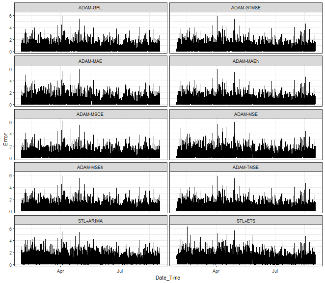
Multivariate Linear Regression Model
As a benchmark, as opposed to catboost, we will try a simple multivariate multiple linear regression model by the base lm function.
You just need to use the cbind function inside the formula to incorporate multiple targets in the model.
mmlm <- lm(as.formula(paste0("cbind(", paste(targets, collapse = ", "), ") ~ .")),
           data = data_predictions_all_casted_train[, .SD, .SDcols = c(targets, features)])

# summary(mmlm)
# manova(mmlm)
# confint(mmlm)
# coef(mmlm)
Summaries of the model would be very large to print here, so I commented on the most useful functions to do your analysis of the trained model with summary, manova, coef, and confint.
Now, let’s predict errors on our selected test set and compute directly prediction errors and Rank accuracy.
mmlm_predicted <- predict(mmlm, data_predictions_all_casted_test[, .SD, .SDcols = c(features)])
dt_mmlm_predicted <- copy(data_predictions_all_casted_test[, .SD, .SDcols = c("Date_Time", targets)])
dt_mmlm_predicted[, (paste0(targets, "_prediction")) := as.data.table(mmlm_predicted)]

dt_mmlm_predicted_melt <- copy(melt(dt_mmlm_predicted,
                                    id.vars = "Date_Time",
                                    measure.vars = list(real = targets,
                                                        predicted = paste0(targets, "_prediction")),
                                    variable.name = "model",
                                    variable.factor = F))

dt_mmlm_predicted_melt[data.table(model = as.character(1:10),
                                  model_name = targets),
                       on = .(model),
                       model := i.model_name]

setorder(dt_mmlm_predicted_melt, Date_Time, real)
dt_mmlm_predicted_melt[, Rank := 1:.N, by = .(Date_Time)]
setorder(dt_mmlm_predicted_melt, Date_Time, predicted)
dt_mmlm_predicted_melt[, Rank_pred := 1:.N, by = .(Date_Time)]

dt_mmlm_predicted_melt[, .(RMSE = round(rmse(real, predicted), 3),
                           MAE = round(mae(real, predicted), 3),
                           MdAE = round(mdae(real, predicted), 3),
                           Rank_error = round(mae(Rank, Rank_pred), 3),
                           Rank_1_accuracy = round(.SD[Rank_pred == 1 & Rank_pred == Rank, .N] / .SD[Rank == 1, .N], 3),
                           Rank_1_cases = .SD[Rank == 1, .N]),
                       by  = .(model)][order(-Rank_1_cases)]
## model RMSE MAE MdAE Rank_error Rank_1_accuracy Rank_1_cases
## 1: Error_STL_ETS 0.476 0.324 0.239 3.149 0.314 892
## 2: Error_ADAM_MSCE 0.429 0.276 0.191 2.766 0.279 634
## 3: Error_ADAM_MAEh 0.443 0.289 0.207 2.768 0.367 621
## 4: Error_STL_ARIMA 0.459 0.308 0.228 2.976 0.223 588
## 5: Error_ADAM_MAE 0.453 0.307 0.226 3.474 0.466 584
## 6: Error_ADAM_MSE 0.448 0.305 0.224 3.303 0.011 379
## 7: Error_ADAM_MSEh 0.420 0.270 0.192 1.985 0.009 212
## 8: Error_ADAM_GPL 0.415 0.266 0.190 2.106 0.097 185
## 9: Error_ADAM_GTMSE 0.419 0.267 0.188 2.045 0.012 82
## 10: Error_ADAM_TMSE 0.420 0.269 0.191 2.060 0.000 47dt_mmlm_predicted_melt[, .(RMSE = rmse(real, predicted),
MAE = mae(real, predicted),
MdAE = mdae(real, predicted),
Rank_error = mae(Rank, Rank_pred),
Rank_1_accuracy = .SD[Rank_pred == 1 & Rank_pred == Rank, .N] / .SD[Rank == 1, .N])]## RMSE MAE MdAE Rank_error Rank_1_accuracy
## 1: 0.4387276 0.2880984 0.2051204 2.662926 0.2634943We can see that the best MAEs have GTMSE, TMSE, and GPL losses. On the other hand, best Rank estimation has MSEh loss and best first Rank estimation accuracy has simple MAE loss method. In general, we miss Rank on average by 2.6 from 10 possible ranks.
Let’s see error predictions from four of our methods.
ggplot(dt_mmlm_predicted_melt[.(targets[c(1,3,5,9)]), on = .(model)],
       aes(Date_Time, predicted, color = "predicted error")) +
  facet_wrap(~model) +
  geom_line(data = dt_mmlm_predicted_melt[.(targets[c(1,3,5,9)]), on = .(model)],
            aes(Date_Time, real, color = "real error")) +
  geom_line(alpha = 0.7, linewidth = 0.6) +
  scale_color_manual(values = c("red", "black")) +
  theme_bw() +
  theme(legend.position="bottom")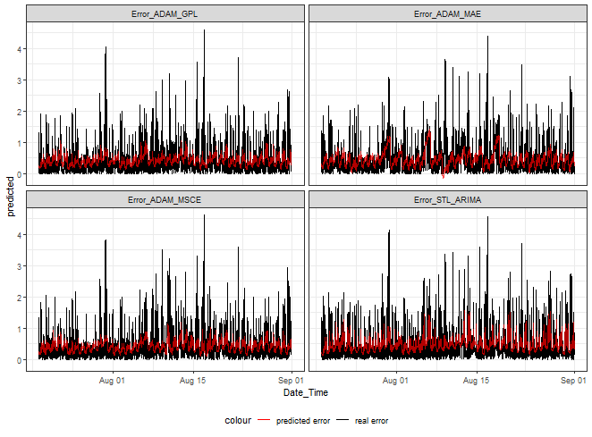
At first sight, it can be seen that we can nicely hit low and medium magnitudes of errors. Again, as shown in my previous post, higher values can’t be predicted.
Shrinkage - LASSO with full interactions
As the second multivariate model benchmark, I will try LASSO (glmnet) shrinkage capability and use all possible interactions to model (by using .^2 in the formula).
lambdas <- 10^seq(3, -2, by = -.1)

data_with_interactions <- model.matrix(~ . + .^2,
                                       data = data_predictions_all_casted_train[, .SD,
                                                                                .SDcols = c(features)])

mlassom <- cv.glmnet(x = data_with_interactions,
                     y = as.matrix(data_predictions_all_casted_train[, .SD, .SDcols = c(targets)]),
                     family = "mgaussian",
                     alpha = 1,
                     lambda = lambdas,
                     intercept = T,
                     standardize = T)
To check estimated coefficients, we can use the predict method.
coefs <- predict(mlassom, type = "coefficients",
                 s = c(mlassom$lambda.min))

mlassom$lambda.min
## [1] 0.01Let’s predict errors on the test set and compute prediction errors.
mlassom_prediction <- predict(mlassom,
                              type = "response",
                              s = mlassom$lambda.min,
                              newx = model.matrix(~ . + .^2,
                                                  data = data_predictions_all_casted_test[, .SD,
                                                                                          .SDcols = c(features)]))

dt_mlassom_predicted <- copy(data_predictions_all_casted_test[, .SD, .SDcols = c("Date_Time", targets)])
dt_mlassom_predicted[, (paste0(targets, "_prediction")) := as.data.table(mlassom_prediction[,,1])]

dt_mlassom_predicted_melt <- copy(melt(dt_mlassom_predicted,
                                       id.vars = "Date_Time",
                                       measure.vars = list(real = targets,
                                                           predicted = paste0(targets, "_prediction")),
                                       variable.name = "model",
                                       variable.factor = F))

dt_mlassom_predicted_melt[data.table(model = as.character(1:10),
                                     model_name = targets),
                          on = .(model),
                          model := i.model_name]

setorder(dt_mlassom_predicted_melt, Date_Time, real)
dt_mlassom_predicted_melt[, Rank := 1:.N, by = .(Date_Time)]
setorder(dt_mlassom_predicted_melt, Date_Time, predicted)
dt_mlassom_predicted_melt[, Rank_pred := 1:.N, by = .(Date_Time)]

dt_mlassom_predicted_melt[, .(RMSE = round(rmse(real, predicted), 3),
                              MAE = round(mae(real, predicted), 3),
                              MdAE = round(mdae(real, predicted), 3),
                              Rank_error = round(mae(Rank, Rank_pred), 3),
                              Rank_1_accuracy = round(.SD[Rank_pred == 1 & Rank_pred == Rank, .N] / .SD[Rank == 1, .N], 3),
                              Rank_1_cases = .SD[Rank == 1, .N]),
                          by  = .(model)][order(-Rank_1_cases)]
## model RMSE MAE MdAE Rank_error Rank_1_accuracy Rank_1_cases
## 1: Error_STL_ETS 0.466 0.325 0.257 3.640 0.151 892
## 2: Error_ADAM_MSCE 0.427 0.277 0.190 2.956 0.341 634
## 3: Error_ADAM_MAEh 0.439 0.290 0.211 2.689 0.243 621
## 4: Error_STL_ARIMA 0.455 0.313 0.239 3.153 0.105 588
## 5: Error_ADAM_MAE 0.447 0.315 0.240 3.208 0.158 584
## 6: Error_ADAM_MSE 0.439 0.306 0.229 3.313 0.003 379
## 7: Error_ADAM_MSEh 0.414 0.263 0.185 2.528 0.019 212
## 8: Error_ADAM_GPL 0.410 0.261 0.182 2.708 0.103 185
## 9: Error_ADAM_GTMSE 0.414 0.261 0.179 2.502 0.134 82
## 10: Error_ADAM_TMSE 0.415 0.264 0.184 2.608 0.064 47dt_mlassom_predicted_melt[, .(RMSE = rmse(real, predicted),
MAE = mae(real, predicted),
MdAE = mdae(real, predicted),
Rank_error = mae(Rank, Rank_pred),
Rank_1_accuracy = .SD[Rank_pred == 1 & Rank_pred == Rank, .N] / .SD[Rank == 1, .N])]## RMSE MAE MdAE Rank_error Rank_1_accuracy
## 1: 0.4328982 0.287333 0.2033996 2.93054 0.1642992We can see that the best MAEs have the same methods as with MMLM. On the other hand, best Rank estimation has GTMSE loss and best first Rank estimation accuracy has MSCE multistep loss method. In general, we miss Rank on average by 2.9 from 10 possible ranks, so worse by 0.3 as opposed to MMLM. We can say that LASSO didn’t much help to our error modeling.
But, let’s see LASSO error predictions from four of our methods.
ggplot(dt_mlassom_predicted_melt[.(targets[c(1,3,5,9)]), on = .(model)],
       aes(Date_Time, predicted, color = "predicted error")) +
  facet_wrap(~model) +
  geom_line(data = dt_mlassom_predicted_melt[.(targets[c(1,3,5,9)]), on = .(model)],
            aes(Date_Time, real, color = "real error")) +
  geom_line(alpha = 0.7, linewidth = 0.6) +
  scale_color_manual(values = c("red", "black")) +
  theme_bw() +
  theme(legend.position="bottom")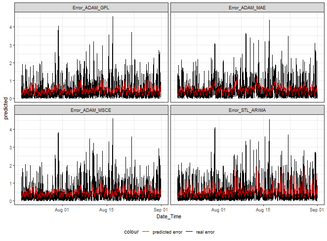
Catboost MultiRMSE
The final multivariate regression method used will be Catboost gradient boosting trees with Multi-target regression loss - MultiRMSE, you can check documentation for this loss here: https://catboost.ai/en/docs/concepts/loss-functions-multiregression.
Let’s define the training method with early stopping based on the validation set and directly train on our dataset.
train_catboost_multirmse <- function(data, target, ncores, valid_ratio) {

  data <- na.omit(data)

  n_rows <- nrow(data)
  idx <- 1:n_rows

  end_ratio <- 0.02
  train_idx <- c(idx[1:floor(n_rows*(1 - (end_ratio + valid_ratio)))],
                 idx[(floor(n_rows*(1-end_ratio)) + 1):n_rows])
  valid_idx <- c(idx[(floor(n_rows*(1 - (end_ratio + valid_ratio)))+1):floor(n_rows*(1-end_ratio))])

  train_pool <- catboost::catboost.load_pool(as.data.frame(data[train_idx, !target, with = F]),
                                             label = as.matrix(data[train_idx, mget(target)]))

  valid_pool <- catboost::catboost.load_pool(as.data.frame(data[valid_idx, !target, with = F]),
                                             label = as.matrix(data[valid_idx, mget(target)]))

  fit_params <- list(iterations = 3000,
                     learning_rate = 0.015,
                     depth = 12,
                     loss_function = 'MultiRMSE',
                     langevin = TRUE,
                     min_data_in_leaf = 5,
                     eval_metric = "MultiRMSE",
                     metric_period = 50,
                     early_stopping_rounds = 60,
                     rsm = 0.75,
                     l2_leaf_reg = 1,
                     train_dir = "train_dir",
                     logging_level = "Verbose",
                     boosting_type = "Plain",
                     grow_policy = "Lossguide",
                     score_function = "L2",
                     bootstrap_type = "Bayesian",
                     bagging_temperature = 1,
                     use_best_model = T,
                     allow_writing_files = F,
                     thread_count = ncores)

  m_cat <- catboost::catboost.train(learn_pool = train_pool,
                                    test_pool = valid_pool,
                                    params = fit_params)

  return(m_cat)

}

m_catboost_multirmse <- train_catboost_multirmse(data = data_predictions_all_casted_train[, .SD, .SDcols = c(targets, features)],
                                                 target = targets,
                                                 ncores = 4,
                                                 valid_ratio = 0.05)
## Warning: Overfitting detector is active, thus evaluation metric is calculated on every iteration. 'metric_period' is ignored for evaluation metric.
## 0: learn: 1.8651752 test: 1.6317912 best: 1.6317912 (0) total: 7.09ms remaining: 21.3s
## 50: learn: 1.7805225 test: 1.4486824 best: 1.4486824 (50) total: 422ms remaining: 24.4s
## 100: learn: 1.7326169 test: 1.3486589 best: 1.3486589 (100) total: 860ms remaining: 24.7s
## 150: learn: 1.7030793 test: 1.2922393 best: 1.2922393 (150) total: 1.35s remaining: 25.5s
## 200: learn: 1.6875372 test: 1.2686592 best: 1.2686592 (200) total: 1.82s remaining: 25.3s
## 250: learn: 1.6747041 test: 1.2518136 best: 1.2518136 (250) total: 2.35s remaining: 25.8s
## 300: learn: 1.6645811 test: 1.2407228 best: 1.2407228 (300) total: 2.9s remaining: 26s
## 350: learn: 1.6557448 test: 1.2312354 best: 1.2312354 (350) total: 3.5s remaining: 26.4s
## 400: learn: 1.6464796 test: 1.2225415 best: 1.2225415 (400) total: 4.17s remaining: 27s
## 450: learn: 1.6404967 test: 1.2173237 best: 1.2173036 (449) total: 4.79s remaining: 27s
## 500: learn: 1.6353707 test: 1.2138953 best: 1.2138953 (500) total: 5.42s remaining: 27s
## 550: learn: 1.6321053 test: 1.2113879 best: 1.2113879 (550) total: 5.96s remaining: 26.5s
## 600: learn: 1.6273276 test: 1.2084719 best: 1.2083969 (599) total: 6.6s remaining: 26.4s
## 650: learn: 1.6235998 test: 1.2067629 best: 1.2067526 (648) total: 7.22s remaining: 26s
## 700: learn: 1.6207368 test: 1.2056776 best: 1.2056776 (700) total: 7.78s remaining: 25.5s
## 750: learn: 1.6178637 test: 1.2046009 best: 1.2045980 (747) total: 8.38s remaining: 25.1s
## 800: learn: 1.6151604 test: 1.2039642 best: 1.2039435 (796) total: 8.99s remaining: 24.7s
## 850: learn: 1.6122595 test: 1.2028463 best: 1.2028463 (850) total: 9.6s remaining: 24.2s
## 900: learn: 1.6101196 test: 1.2020336 best: 1.2019819 (890) total: 10.2s remaining: 23.7s
## 950: learn: 1.6073753 test: 1.2011880 best: 1.2011371 (948) total: 10.8s remaining: 23.3s
## 1000: learn: 1.6052842 test: 1.2006492 best: 1.2006411 (999) total: 11.4s remaining: 22.8s
## 1050: learn: 1.6039241 test: 1.2001930 best: 1.2001853 (1049) total: 12s remaining: 22.2s
## 1100: learn: 1.6028500 test: 1.1999358 best: 1.1999358 (1100) total: 12.5s remaining: 21.5s
## 1150: learn: 1.6012678 test: 1.1992978 best: 1.1992978 (1150) total: 13.2s remaining: 21.2s
## 1200: learn: 1.5997241 test: 1.1989927 best: 1.1989927 (1200) total: 13.8s remaining: 20.7s
## 1250: learn: 1.5984334 test: 1.1989688 best: 1.1989617 (1248) total: 14.5s remaining: 20.3s
## 1300: learn: 1.5969307 test: 1.1986201 best: 1.1985152 (1278) total: 15.2s remaining: 19.9s
## 1350: learn: 1.5948609 test: 1.1986032 best: 1.1985116 (1314) total: 15.9s remaining: 19.4s
## Stopped by overfitting detector (60 iterations wait)
##
## bestTest = 1.198511627
## bestIteration = 1314
##
## Shrink model to first 1315 iterations.m_catboost_multirmse## CatBoost model (1315 trees)
## Loss function: MultiRMSE
## Fit to 14 feature(s)We can check the Feature Importance of the trained model:
fea_imp_catboost <- catboost::catboost.get_feature_importance(m_catboost_multirmse)
fea_imp_catboost <- data.table::data.table(Gain = fea_imp_catboost[,1],
                                           Feature = features)
setorder(fea_imp_catboost, -Gain)
fea_imp_catboost
## Gain Feature
## 1: 26.2825537 Load_predicted_STL_ETS
## 2: 10.2856293 Load_predicted_ADAM_MAE
## 3: 8.9606314 Load_predicted_ADAM_GPL
## 4: 8.5230838 Load_predicted_ADAM_MSCE
## 5: 8.4006334 Load_predicted_ADAM_GTMSE
## 6: 6.5706169 Load_predicted_ADAM_TMSE
## 7: 6.2375988 Load_predicted_STL_ARIMA
## 8: 5.0254951 Load_predicted_ADAM_MSEh
## 9: 4.8948488 S_day
## 10: 4.7176922 Load_predicted_ADAM_MSE
## 11: 3.8361990 Load_predicted_ADAM_MAEh
## 12: 3.3433404 C_week
## 13: 2.2428758 C_day
## 14: 0.6788015 S_weekSTL_ETS and MAE simple loss predictions have the highest importance to the multivariate model.
Let’s predict the test set and compute prediction errors.
predict_multirmse_catboost <- function(data, target, cat_model) {

  pred <- catboost::catboost.predict(cat_model,
                                     catboost::catboost.load_pool(as.data.frame(data),
                                                                  label = as.matrix(rep(0, nrow(data)), ncol = length(target))
                                     ),
                                     thread_count = 1)

  return(pred)

}

catboost_prediction <- predict_multirmse_catboost(data = data_predictions_all_casted_test[, .SD, .SDcols = c(features)],
                                                  target = targets,
                                                  cat_model = m_catboost_multirmse)

dt_catboost_predicted <- copy(data_predictions_all_casted_test[, .SD, .SDcols = c("Date_Time", targets)])
dt_catboost_predicted[, (paste0(targets, "_prediction")) := as.data.table(catboost_prediction)]

dt_catboost_predicted_melt <- copy(melt(dt_catboost_predicted,
                                        id.vars = "Date_Time",
                                        measure.vars = list(real = targets,
                                                            predicted = paste0(targets, "_prediction")),
                                        variable.name = "model",
                                        variable.factor = F))

dt_catboost_predicted_melt[data.table(model = as.character(1:10),
                                      model_name = targets),
                           on = .(model),
                           model := i.model_name]

setorder(dt_catboost_predicted_melt, Date_Time, real)
dt_catboost_predicted_melt[, Rank := 1:.N, by = .(Date_Time)]
setorder(dt_catboost_predicted_melt, Date_Time, predicted)
dt_catboost_predicted_melt[, Rank_pred := 1:.N, by = .(Date_Time)]

dt_catboost_predicted_melt[, .(RMSE = round(rmse(real, predicted), 3),
                               MAE = round(mae(real, predicted), 3),
                               MdAE = round(mdae(real, predicted), 3),
                               Rank_error = round(mae(Rank, Rank_pred), 3),
                               Rank_1_accuracy = round(.SD[Rank_pred == 1 & Rank_pred == Rank, .N] / .SD[Rank == 1, .N], 3),
                               Rank_1_cases = .SD[Rank == 1, .N]),
                           by  = .(model)][order(-Rank_1_cases)]
## model RMSE MAE MdAE Rank_error Rank_1_accuracy Rank_1_cases
## 1: Error_STL_ETS 0.467 0.307 0.213 3.428 0.367 892
## 2: Error_ADAM_MSCE 0.430 0.273 0.178 2.996 0.181 634
## 3: Error_ADAM_MAEh 0.440 0.280 0.187 2.920 0.072 621
## 4: Error_STL_ARIMA 0.456 0.291 0.195 3.262 0.315 588
## 5: Error_ADAM_MAE 0.449 0.305 0.218 3.229 0.166 584
## 6: Error_ADAM_MSE 0.440 0.293 0.204 3.209 0.021 379
## 7: Error_ADAM_MSEh 0.415 0.252 0.158 2.458 0.042 212
## 8: Error_ADAM_GPL 0.411 0.249 0.155 2.626 0.049 185
## 9: Error_ADAM_GTMSE 0.415 0.248 0.153 2.417 0.024 82
## 10: Error_ADAM_TMSE 0.416 0.251 0.157 2.008 0.000 47dt_catboost_predicted_melt[, .(RMSE = rmse(real, predicted),
MAE = mae(real, predicted),
MdAE = mdae(real, predicted),
Rank_error = mae(Rank, Rank_pred),
Rank_1_accuracy = .SD[Rank_pred == 1 & Rank_pred == Rank, .N] / .SD[Rank == 1, .N])]## RMSE MAE MdAE Rank_error Rank_1_accuracy
## 1: 0.4343794 0.2748845 0.1785648 2.855114 0.1886837We can see that the MAE and MdAE metrics were improved by catboost. On the other hand, average Rank estimation and first Rank estimation are not better than with MMLM.
Let’s plot our predicted errors.
ggplot(dt_catboost_predicted_melt[.(targets[c(1,3,5,9)]), on = .(model)],
       aes(Date_Time, predicted, color = "predicted error")) +
  facet_wrap(~model) +
  geom_line(data = dt_catboost_predicted_melt[.(targets[c(1,3,5,9)]), on = .(model)],
            aes(Date_Time, real, color = "real error")) +
  geom_line(alpha = 0.7, linewidth = 0.6) +
  scale_color_manual(values = c("red", "black")) +
  theme_bw() +
  theme(legend.position="bottom")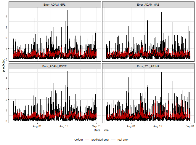
Models analysis
To have it nicely together, let’s bind all three models’ predictions and compute prediction errors for models and methods.
dt_all_predicted <- rbindlist(list(dt_mmlm_predicted_melt[, method := "mmlm"],
                                   dt_mlassom_predicted_melt[, method := "mlasso"],
                                   dt_catboost_predicted_melt[, method := "catboost"]),
                              use.names = T, fill = T)

dt_all_predicted[, Error := real - predicted]
dt_all_predicted[, AE := abs(Error)]

dt_all_predicted[, .(RMSE = rmse(real, predicted),
                     MAE = mae(real, predicted),
                     MdAE = mdae(real, predicted),
                     Rank_error = mae(Rank, Rank_pred),
                     Rank_1_accuracy = .SD[Rank_pred == 1 & Rank_pred == Rank, .N] / .SD[Rank == 1, .N]),
                 by = .(method)][order(MAE)]
## method RMSE MAE MdAE Rank_error Rank_1_accuracy
## 1: catboost 0.4343794 0.2748845 0.1785648 2.855114 0.1886837
## 2: mlasso 0.4328982 0.2873330 0.2033996 2.930540 0.1642992
## 3: mmlm 0.4387276 0.2880984 0.2051204 2.662926 0.2634943dt_all_predicted[, .(RMSE = rmse(real, predicted),
MAE = mae(real, predicted),
MdAE = mdae(real, predicted),
Rank_error = mae(Rank, Rank_pred),
Rank_1_accuracy = .SD[Rank_pred == 1 & Rank_pred == Rank, .N] / .SD[Rank == 1, .N]),
by = .(model)][order(Rank_error)]## model RMSE MAE MdAE Rank_error Rank_1_accuracy
## 1: Error_ADAM_TMSE 0.4172927 0.2610935 0.1773354 2.225221 0.02127660
## 2: Error_ADAM_GTMSE 0.4161971 0.2587184 0.1728826 2.321023 0.05691057
## 3: Error_ADAM_MSEh 0.4161620 0.2616851 0.1787479 2.323469 0.02358491
## 4: Error_ADAM_GPL 0.4119315 0.2586888 0.1757232 2.479640 0.08288288
## 5: Error_ADAM_MAEh 0.4407660 0.2861382 0.2026681 2.792456 0.22758991
## 6: Error_ADAM_MSCE 0.4286877 0.2752749 0.1868000 2.906013 0.26708728
## 7: Error_STL_ARIMA 0.4566267 0.3042826 0.2207566 3.130051 0.21428571
## 8: Error_ADAM_MSE 0.4423139 0.3010806 0.2195689 3.274779 0.01143360
## 9: Error_ADAM_MAE 0.4496008 0.3087655 0.2274286 3.303741 0.26312785
## 10: Error_STL_ETS 0.4697423 0.3186589 0.2340111 3.405540 0.27727952As already mentioned, the best multivariate regression model based on classical prediction metrics is catboosts MultiRMSE. On the other hand, the best model based on right Rank estimation is simple multivariate linear regression.
Let’s do some basic model analysis and see a boxplot of absolute errors.
ggplot(dt_all_predicted[.(targets[c(1, 3, 5, 9)]), on = .(model)],
       aes(method, AE, fill = method)) +
  geom_boxplot() +
  theme_bw()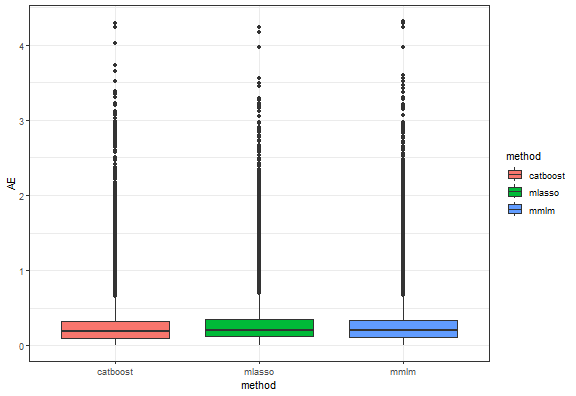
Predicted vs. real values scatter plot:
ggplot(dt_all_predicted[.(targets[c(1, 3, 5, 9)]), on = .(model)],
       aes(predicted, real)) +
  facet_wrap(~method, scales = "fixed", ncol = 3) +
  geom_point(alpha = 0.5) +
  geom_abline(intercept = 0, slope = 1, color = "red",
              linetype = "dashed", linewidth = 1) +
  geom_smooth(alpha = 0.4) +
  labs(title = "Predicted vs Real values") +
  theme_bw()
## `geom_smooth()` using method = 'gam' and formula = 'y ~ s(x, bs = "cs")'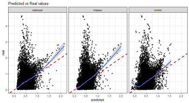
Errors vs. real values scatter plot:
ggplot(dt_all_predicted[.(targets[c(1, 3, 5, 9)]), on = .(model)],
       aes(Error, real)) +
  facet_wrap(~method, scales = "fixed", ncol = 3) +
  geom_point(alpha = 0.5) +
  geom_smooth(alpha = 0.6) +
  xlab("resid (predicted_value - real_value)") +
  labs(title = "Residual vs Real values") +
  theme_bw()
## `geom_smooth()` using method = 'gam' and formula = 'y ~ s(x, bs = "cs")'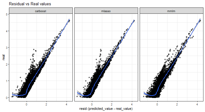
And heteroscedasticity check, so absolute errors vs. real values:
ggplot(dt_all_predicted[.(targets[c(1, 3, 5, 9)]), on = .(model)],
       aes(real, AE)) +
  facet_wrap(~method, scales = "free") +
  geom_point(alpha = 0.5) +
  geom_smooth(alpha = 0.6) +
  ylab("abs(resid)") +
  labs(title = "Heteroscedasticity check") +
  theme_bw()
## `geom_smooth()` using method = 'gam' and formula = 'y ~ s(x, bs = "cs")'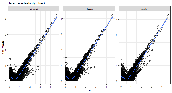
From all the above graphs, we can see that low and medium magnitudes of errors can be nicely predicted, but again prediction of high values of errors is a very difficult task.
We can use nonparametric multiple comparisons test (Nemenyi test) also to decide which error model is best (by Absolute Errors - AE).
tsutils::nemenyi(data.matrix(dcast(dt_all_predicted,
                                   Date_Time + model ~ method,
                                   value.var = "AE")[, !c("Date_Time", "model"), with = F]),
                 plottype = "vmcb")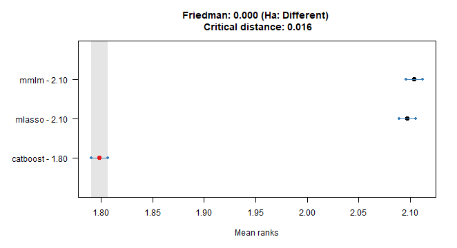
## Friedman and Nemenyi Tests
## The confidence level is 5%
## Number of observations is 42240 and number of methods is 3
## Friedman test p-value: 0.0000 - Ha: Different
## Critical distance: 0.0161
Catboost is best all the way.
We can also use the Nemenyi test on a question that which of the 10 model errors can be predicted the best.
tsutils::nemenyi(data.matrix(dcast(dt_all_predicted,
                                   Date_Time + method ~ model,
                                   value.var = "AE")[, !c("Date_Time", "method"), with = F]),
                 plottype = "vmcb")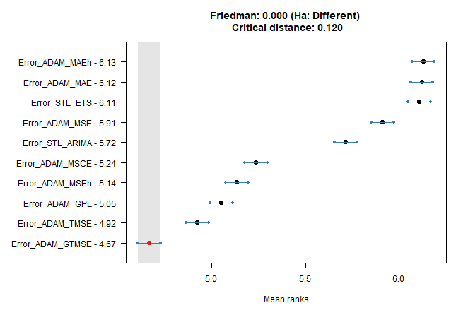
## Friedman and Nemenyi Tests
## The confidence level is 5%
## Number of observations is 12672 and number of methods is 10
## Friedman test p-value: 0.0000 - Ha: Different
## Critical distance: 0.1203
We see that GTMSE and TMSE have the most predictable errors, for non-multistep losses methods (benchmarks) it is more difficult.
Ensemble predictions
Finally, we can now construct some ensemble predictions by our multivariate error model predictions.
Best Rank prediction ensemble
The first method will be very simple, we will use as final ensemble prediction the prediction with the lowest estimated error.
dt_all_predicted[, model := gsub("Error_", "", model)]
data_best_rank_prediction <- copy(dt_all_predicted[, .SD[Rank_pred == 1], by = .(method, Date_Time)])
data_best_rank_prediction[, table(model)] # distribution of used methods
## model
## ADAM_GPL ADAM_GTMSE ADAM_MAE ADAM_MAEh ADAM_MSCE ADAM_MSE ADAM_MSEh
## 899 880 1513 1613 2302 204 322
## ADAM_TMSE STL_ARIMA STL_ETS
## 279 1713 2947Let’s evaluate ensemble predictions by our error models and also compute metrics for our base predictions for comparison.
data_predictions_all[, model := gsub("-", "_", model)]
data_predictions_all[, model := gsub("\\+", "_", model)]

data_best_rank_prediction[data_predictions_all,
                          on = .(model, Date_Time),
                          Load_predicted := i.Load_predicted]

data_best_rank_prediction[data_predictions_all,
                          on = .(Date_Time),
                          Load_real := i.Load_real]

# original
data_predictions_all[Date_Time %in% data_best_rank_prediction[, unique(Date_Time)],
                     .(RMSE = rmse(Load_real, Load_predicted),
                       MAE = mae(Load_real, Load_predicted),
                       MAAPE = maape(Load_real, Load_predicted)),
                     by = .(model)][order(MAE)]
## model RMSE MAE MAAPE
## 1: ADAM_MAEh 0.6153573 0.3915900 79.73346
## 2: ADAM_MSEh 0.6060004 0.4032142 84.61694
## 3: ADAM_TMSE 0.6080947 0.4053491 84.76779
## 4: ADAM_GTMSE 0.6094993 0.4085337 85.40032
## 5: ADAM_GPL 0.6082200 0.4106951 85.66970
## 6: ADAM_MSCE 0.6251760 0.4153277 85.63160
## 7: STL_ARIMA 0.6709538 0.4348279 87.92342
## 8: ADAM_MSE 0.6487472 0.4378956 87.45296
## 9: ADAM_MAE 0.6550635 0.4386036 87.33271
## 10: STL_ETS 0.6887292 0.4388718 80.82078# ensemble
data_best_rank_prediction[, .(RMSE = rmse(Load_real, Load_predicted),
MAE = mae(Load_real, Load_predicted),
MAAPE = maape(Load_real, Load_predicted)),
by = .(method)][order(MAE)]## method RMSE MAE MAAPE
## 1: catboost 0.6176298 0.3765020 78.38730
## 2: mmlm 0.6368562 0.3777519 76.25634
## 3: mlasso 0.6090476 0.3789960 81.54793All three ensembles are better than any base prediction based on MAE. Well done!
Let’s plot a graph of the final ensemble predictions:
ggplot(data_best_rank_prediction,
       aes(Date_Time, Load_predicted, color = "predicted load")) +
  facet_wrap(~method, ncol = 1) +
  geom_line(data = data_best_rank_prediction,
            aes(Date_Time, Load_real, color = "real load")) +
  geom_line(alpha = 0.7, linewidth = 0.6) +
  scale_color_manual(values = c("red", "black")) +
  theme_bw() +
  theme(legend.position="bottom")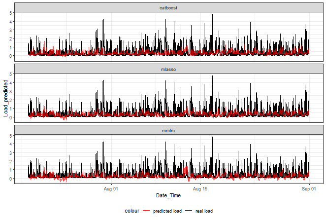
Catboost doesn’t go that much below zero than the other two.
Weighted average Ensemble
The second ensemble method will be based on weighting the estimated errors. Firstly, we need to normalize all weights (errors) by the Min-max method and compute the sum ratio.
weis <- copy(dt_all_predicted[, .(Wei_m = TSrepr::norm_min_max(-abs(predicted)),
                                  model),
                             by = .(method, Date_Time)])

weis_sums <- copy(dt_all_predicted[, .(Wei_sum = sum(TSrepr::norm_min_max(-abs(predicted)))),
                                   by = .(method, Date_Time)])

weis[weis_sums,
     Wei_m := Wei_m / i.Wei_sum,
     on = .(method, Date_Time)]
We can use all predictions, but a better way is to remove the bad half of the predictions from the ensemble:
ratio_forec <- 0.5 # 1 to use all 10 predictions
setorder(weis, method, Date_Time, Wei_m)
weis[, Wei_m := replace(Wei_m, 1:floor(.N * ratio_forec), 0),
     by = .(method, Date_Time)]
Now, let’s join weights and predictions and compute final ensemble predictions.
dt_all_predicted_wei_ave <- copy(dt_all_predicted)
dt_all_predicted_wei_ave[weis,
                         Wei_m := i.Wei_m,
                         on = .(model, method, Date_Time)]

dt_all_predicted_wei_ave[data_predictions_all,
                         on = .(model, Date_Time),
                         Load_predicted := i.Load_predicted]

data_predicted_wei_ave <- copy(dt_all_predicted_wei_ave[,
                                                        .(Load_predicted = weighted.mean(Load_predicted, Wei_m)),
                                                        by = .(method, Date_Time)])
Let’s evaluate them:
data_predicted_wei_ave[data_predictions_all,
                       on = .(Date_Time),
                       Load_real := i.Load_real]

data_predicted_wei_ave[, .(RMSE = rmse(Load_real, Load_predicted),
                           MAE = mae(Load_real, Load_predicted),
                           MAAPE = maape(Load_real, Load_predicted)),
                       by = .(method)][order(MAE)]
## method RMSE MAE MAAPE
## 1: mmlm 0.6080235 0.3721450 78.36590
## 2: catboost 0.6027960 0.3814034 82.43628
## 3: mlasso 0.5981348 0.3824002 81.68486Even better with weighting than the best rank way!
Let’s plot a graph of ensemble predictions:
ggplot(data_predicted_wei_ave,
       aes(Date_Time, Load_predicted, color = "predicted load")) +
  facet_wrap(~method, ncol = 1) +
  geom_line(data = data_predicted_wei_ave,
            aes(Date_Time, Load_real, color = "real load")) +
  geom_line(alpha = 0.7, linewidth = 0.6) +
  scale_color_manual(values = c("red", "black")) +
  theme_bw() +
  theme(legend.position="bottom")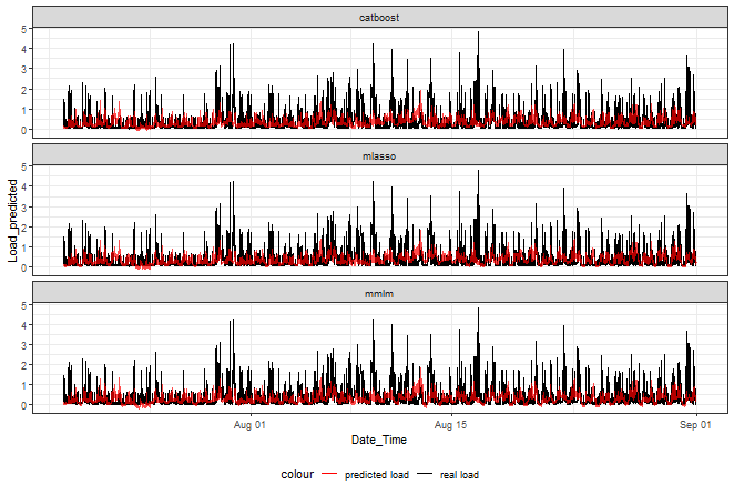
Ultimately, let’s decide which model is best for household electricity consumption prediction:
data_predictions_all_ensembles <- rbindlist(list(data_predictions_all[Date_Time %in% data_best_rank_prediction[, unique(Date_Time)], .(Date_Time, Load_predicted, Load_real, model)],
                                                 data_predicted_wei_ave[, .(Date_Time, Load_predicted, Load_real, model = paste0("ensemble_wei_ave_", method))],
                                                 data_best_rank_prediction[, .(Date_Time, Load_predicted, Load_real, model = paste0("ensemble_best_rank_", method))]))

data_predictions_all_ensembles[, AE := abs(Load_real - Load_predicted)]

tsutils::nemenyi(data.matrix(dcast(data_predictions_all_ensembles,
                                   Date_Time ~ model,
                                   value.var = "AE")[, !c("Date_Time"), with = F]),
                 plottype = "vmcb")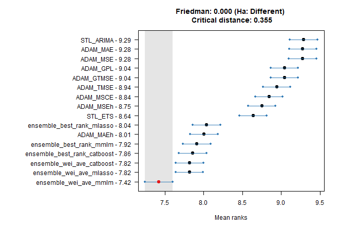
## Friedman and Nemenyi Tests
## The confidence level is 5%
## Number of observations is 4224 and number of methods is 16
## Friedman test p-value: 0.0000 - Ha: Different
## Critical distance: 0.3549
Weighted average ensemble prediction using the MMLM method is best!
Summary
- I showed how easily can be modeled multiple targets with three methods: MMLM, LASSO, and Catboost in R
- I trained a model for predicting absolute errors of mostly simple exponential smoothing methods
- The multivariate models can nicely predict errors of low-medium magnitude
- Again the high errors can not be predicted with those simple models
- Catboost showed the best results in regard of absolute error measure
- I used predicted errors to create two types of ensemble predictions of electricity consumption
- Both ensemble methods showed better results than any original prediction
Seven coffees were consumed while writing this article.
If you’ve found it valuable, please consider supporting my work and...
