Multistep horizon loss optimized forecasting with ADAM

Written on 2023-10-26

Recently, during work on some forecasting task at PowereX, I stumbled upon an interesting improvement in time series forecasting modeling. In general, in regression modeling, we use evaluation/loss metrics based on one step ahead (one value) horizon. But, in many forecasting applications, we are interested in multistep horizon forecasting (e.g. whole 1 day ahead), so some multistep losses would be great to optimize during training of forecasting models. Except obviously in some RNN architectures, this wasn’t easily possible in used libraries/frameworks in the past time.

So, I was very happy to see multistep losses in smooth package and its adam() wrapper and to try it. I already used it in one particular task in my work, and it went successfully to production!

My motivation and what I will show you in this blog post is:

Tribute to the smooth package and its adam() wrapper - especially for its multistep horizon forecasting losses.
Try to use the mentioned losses for forecasting household consumption times series -> very noisy with daily/weekly seasons, no trend.
Show model diagnostic methods with ggplot2 visualizations.

Household consumption data

Firstly, let’s load all the needed packages for forecasting.

library(data.table)
library(lubridate)
library(TSrepr)
library(smooth)
library(forecast)
library(ggplot2)

Next, I will read one household electricity consumption load data. There are data from 2023-01-01 to 2023-08-31. This household heats space and water with electricity - so there are multiple seasonalities that vary during the year.

data_household_consumption <- fread("_Rscripts/household_consumption.csv") # Date_Time in CET, Load in kW
str(data_household_consumption)

## Classes 'data.table' and 'data.frame':	23328 obs. of  2 variables:
##  $ Date_Time: POSIXct, format: "2023-01-01 00:00:00" "2023-01-01 00:15:00" "2023-01-01 00:30:00" "2023-01-01 00:45:00" ...
##  $ Load     : num  0.362 0.622 0.435 0.236 0.322 0.565 0.338 0.467 0.639 0.46 ...
##  - attr(*, ".internal.selfref")=<externalptr>

summary(data_household_consumption)

##    Date_Time                        Load       
##  Min.   :2023-01-01 00:00:00   Min.   :0.0000  
##  1st Qu.:2023-03-02 17:56:15   1st Qu.:0.1140  
##  Median :2023-05-02 11:52:30   Median :0.4440  
##  Mean   :2023-05-02 11:52:30   Mean   :0.7468  
##  3rd Qu.:2023-07-02 05:48:45   3rd Qu.:1.1150  
##  Max.   :2023-08-31 23:45:00   Max.   :7.1510

Let’s visualize consumption for one month.

ggplot(data_household_consumption[Date_Time >= as.Date("2023-04-01") & Date_Time <= as.Date("2023-05-01")]) +
  geom_line(aes(Date_Time, Load)) +
  labs(y = "Load (kW)") +
  theme_bw()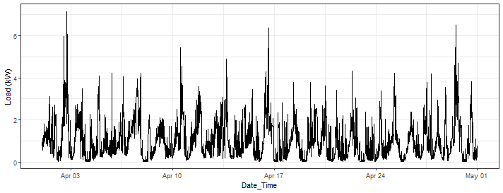

plot of chunk unnamed-chunk-3

We can see that the behavior of the time series is very noisy but with clear daily pattern.

Let’s check more in detail, what we will face during forecasting, so I will show you the weekly average pattern (+/- standard deviation) by month.

data_household_consumption[, week_period := 1:.N, by = .(Week = lubridate::week(Date_Time))]
data_household_consumption[, month := lubridate::month(Date_Time, label = T)]
data_weekly_profiles <- copy(data_household_consumption[, .(Mean = mean(Load),
                                                            SD = sd(Load)),
                                                        by = .(month, week_period)])
 
ggplot(data_weekly_profiles, aes(x = week_period, Mean)) + 
  facet_wrap(~month) +
  geom_ribbon(data = data_weekly_profiles, aes(ymin = Mean - SD, ymax = Mean + SD),
              fill = "firebrick2", alpha = 0.4) +
  geom_line(linewidth = 0.9) + 
  geom_vline(xintercept = c(96, 96*4, 96*5, 96*6), linetype = 2, linewidth = 0.8) +
  theme(title = element_text(size = 14),
        axis.text = element_text(size = 10),
        axis.title = element_text(size = 12, face = "bold")) +
  labs(title = "Mean weekly profile +- deviation (SD)") +
  labs(x = "Time", y = "Load (kW)")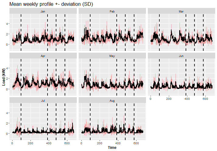

plot of chunk unnamed-chunk-4

We can see that consumption patterns change over months…

I will show you also an average daily pattern by month.

data_household_consumption[, day_period := 1:.N, by = .(Date = date(Date_Time))]
data_daily_profiles <- copy(data_household_consumption[, .(Mean = mean(Load),
                                                            SD = sd(Load)),
                                                        by = .(month, day_period)])
 
ggplot(data_daily_profiles, aes(x = day_period, Mean)) + 
  facet_wrap(~month) +
  geom_ribbon(data = data_daily_profiles, aes(ymin = Mean - SD, ymax = Mean + SD),
              fill = "firebrick2", alpha = 0.4) +
  geom_line(linewidth = 0.9) + 
  theme(title = element_text(size = 14),
        axis.text = element_text(size = 10),
        axis.title = element_text(size = 12, face = "bold")) +
  labs(title = "Mean daily profile +- deviation (SD)") +
  labs(x = "Time", y = "Load (kW)")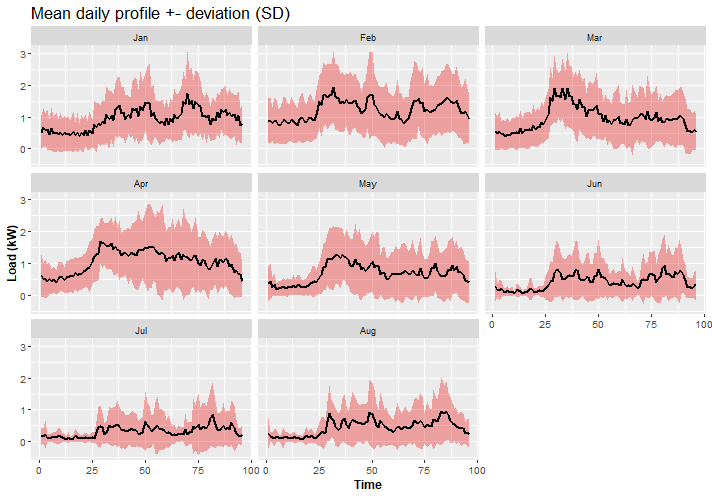

plot of chunk unnamed-chunk-5

It’s obvious that during winter months there is different behavior of electricity consumption, and much more consumed electricity because of heating needs.

smooth and ADAM

The main goal of this blog post is to try experimentally multistep losses in ETS model and compare them against classical losses (MSE and MAE).

In adam function we have several possibilities for multistep losses, check in here: https://openforecast.org/adam/multistepLosses.html.

I will use these in experiments:

MSEh, MAEh
TMSE – Trace MSE
GTMSE – Geometric Trace MSE
MSCE – Mean Squared Cumulative Error
GPL – General Predictive Likelihood

Let’s try adam on 4 weeks sample of data.

win_days <- 28 # 4 weeks
all_dates <- data_household_consumption[, unique(date(Date_Time))]
data_household_consumption_4weeks <- copy(data_household_consumption[Date_Time >= all_dates[1] & Date_Time < all_dates[win_days + 1]])

Firstly, I will try only the additive ETS model with classic MSE loss.

adam_model_classic <- adam(data = data_household_consumption_4weeks[, Load],
                           model = "XXX",
                           lags = c(1, 96, 96*7),
                           loss = "MSE",
                           h = 96,
                           holdout = T,
                           ic = "AICc",
                           initial = "back")
 
adam_model_classic

## Time elapsed: 0.99 seconds
## Model estimated using adam() function: ETS(ANA)[96, 672]
## Distribution assumed in the model: Normal
## Loss function type: MSE; Loss function value: 0.2732
## Persistence vector g:
##  alpha gamma1 gamma2 
## 0.5246 0.0000 0.0791 
## 
## Sample size: 2592
## Number of estimated parameters: 3
## Number of degrees of freedom: 2589
## Information criteria:
##      AIC     AICc      BIC     BICc 
## 3998.436 3998.445 4016.017 4016.053 
## 
## Forecast errors:
## ME: 0.041; MAE: 0.534; RMSE: 0.726
## sCE: 425.014%; Asymmetry: -15.5%; sMAE: 57.586%; sMSE: 61.353%
## MASE: 1.304; RMSSE: 1.2; rMAE: 0.845; rRMSE: 0.897

plot(adam_model_classic, which = 7)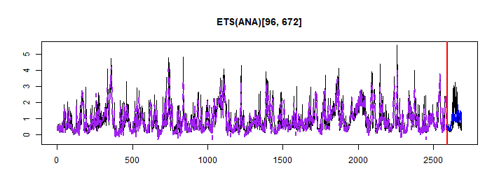

plot of chunk unnamed-chunk-7

We can see that ANA model is selected, so additive on level and season components, trend component was not used.

Let’s try multistep loss - GPL.

adam_model_multistep <- adam(data = data_household_consumption_4weeks[, Load],
                             model = "XXX",
                             lags = c(1, 96, 96*7),
                             loss = "GPL",
                             h = 96,
                             holdout = T,
                             ic = "AICc",
                             initial = "back")
 
adam_model_multistep

## Time elapsed: 25.37 seconds
## Model estimated using adam() function: ETS(ANA)[96, 672]
## Distribution assumed in the model: Normal
## Loss function type: GPL; Loss function value: -135.4807
## Persistence vector g:
##  alpha gamma1 gamma2 
## 0.0004 0.0000 0.0884 
## 
## Sample size: 2592
## Number of estimated parameters: 3
## Number of degrees of freedom: 2589
## Information criteria:
##      AIC     AICc      BIC     BICc 
## 3703.800 3703.809 3721.380 3721.417 
## 
## Forecast errors:
## ME: 0.075; MAE: 0.526; RMSE: 0.732
## sCE: 778.763%; Asymmetry: -7.8%; sMAE: 56.684%; sMSE: 62.332%
## MASE: 1.284; RMSSE: 1.21; rMAE: 0.832; rRMSE: 0.904

plot(adam_model_multistep, which = 7)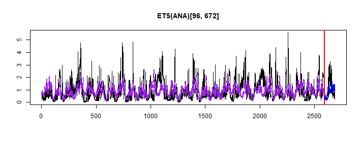

plot of chunk unnamed-chunk-8

Also, ANA was selected. Better AICc and MAE with multistep loss, but RMSE was worse than in the MSE case. Let’s see on whole dataset…

Prediction simulations

I will roll predictions day by day with a whole 1-day prediction horizon with a train-set of length 28 days (win_days) on our household consumption data -> so 214 predictions will be made. I will use all multistep losses mentioned above, MAE, MSE, and STL+ARIMA, STL+ETS methods from the forecast package as benchmarks (as was used also in my previous blog post about bootstrapping). You can check R script how to simulate and compute this in parallel on my GitHub repository.

Now, let’s see generated predictions.

load("_rmd/data_household_predictions.Rdata")
data_predictions_all

##                   Date_Time Load_real Load_predicted    model
##      1: 2023-01-30 00:00:00     0.274     -0.7679345  STL+ETS
##      2: 2023-01-30 00:15:00     0.363     -0.7959601  STL+ETS
##      3: 2023-01-30 00:30:00     0.342     -0.7443988  STL+ETS
##      4: 2023-01-30 00:45:00     0.391     -0.8461708  STL+ETS
##      5: 2023-01-30 01:00:00     0.230     -0.8708582  STL+ETS
##     ---                                                      
## 205436: 2023-08-31 22:45:00     0.080      0.4030999 ADAM-GPL
## 205437: 2023-08-31 23:00:00     0.039      0.2060178 ADAM-GPL
## 205438: 2023-08-31 23:15:00     0.087      0.2489654 ADAM-GPL
## 205439: 2023-08-31 23:30:00     0.080      0.1719251 ADAM-GPL
## 205440: 2023-08-31 23:45:00     0.040      0.4710469 ADAM-GPL

I will compute forecasting evaluation metrics as RMSE, MAE, and MAAPE.

data_predictions_all[, .(RMSE = rmse(Load_real, Load_predicted),
                         MAE = mae(Load_real, Load_predicted),
                         MAAPE = maape(Load_real, Load_predicted)),
                     by = .(model)][order(MAE)]

##          model      RMSE       MAE    MAAPE
##  1:  ADAM-MSCE 0.7645952 0.5588521 77.19498
##  2:  ADAM-MAEh 0.7768230 0.5596729 75.60581
##  3:  ADAM-TMSE 0.7703792 0.5622345 77.03544
##  4:  ADAM-MSEh 0.7713433 0.5623389 76.99981
##  5: ADAM-GTMSE 0.7704186 0.5626845 77.15252
##  6:   ADAM-GPL 0.7704062 0.5629255 77.17820
##  7:   ADAM-MAE 0.8690460 0.6133876 78.18846
##  8:   ADAM-MSE 0.8701501 0.6152678 78.22642
##  9:  STL+ARIMA 0.8751174 0.6159549 78.60016
## 10:    STL+ETS 0.9403524 0.6500436 76.13823

We can see that all multistep losses are better than benchmark methods! That’s very nice results!

For further analysis, we will check only the two best multistep losses and two benchmarks.

models_sub <- c("ADAM-MSCE", "ADAM-MAEh", "ADAM-MAE", "STL+ARIMA")

Let’s see all generated prediction graphs with selected models:

ggplot(data_predictions_all[model %in% models_sub], aes(Date_Time, Load_predicted)) +
  facet_wrap(~model, ncol = 1) +
  geom_line(data = data_predictions_all[model %in% models_sub],
            aes(Date_Time, Load_real),
            color = "black") +
  geom_line(color = "firebrick1") +
  theme_bw()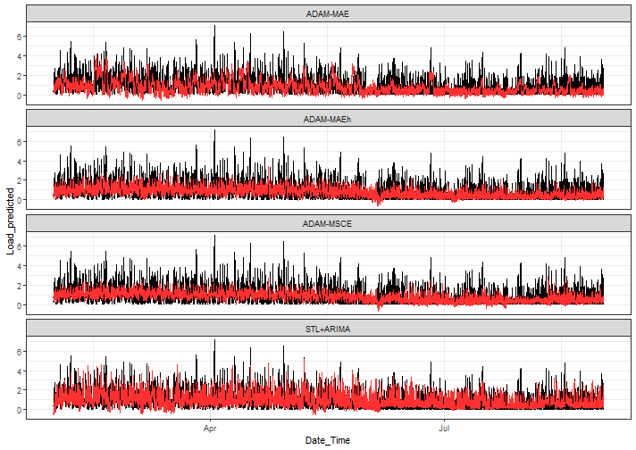

plot of chunk unnamed-chunk-12

There is a much lower variance of predictions with multistep losses ETS than in benchmarks, which’s interesting, but in nature of these losses logical also -> again check https://openforecast.org/adam/multistepLosses.html#multistepLosses.

Models diagnostics

Next, I will try to demonstrate how to compare results from multiple models and analyze them with model diagnostic methods, which are also described in adam forecasting book.

Let’s create residuals and abs(residuals) columns for investigation purposes.

data_predictions_all[, Error := Load_real - Load_predicted]
data_predictions_all[, AE := abs(Error)]

Let’s see the boxplot of absolute errors:

ggplot(data_predictions_all[model %in% models_sub],
       aes(model, AE, fill = model)) +
  geom_boxplot() +
  theme_bw()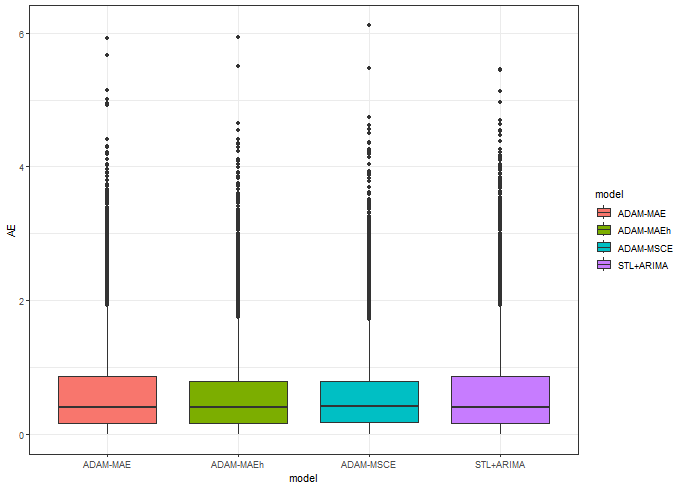

plot of chunk unnamed-chunk-14

We see narrower IQR with multistep losses, that’s a good feature.

Predictions vs real values scatter plot:

ggplot(data_predictions_all[model %in% models_sub],
       aes(Load_predicted, Load_real)) +
  facet_wrap(~model, scales = "fixed", ncol = 2) +
  geom_point(alpha = 0.5) +
  geom_abline(intercept = 0, slope = 1, color = "red", 
              linetype = "dashed", linewidth = 1) +
  geom_smooth(alpha = 0.4) +
  labs(title = "Predicted vs Real values") +
  theme_bw()

## `geom_smooth()` using method = 'gam' and formula = 'y ~ s(x, bs = "cs")'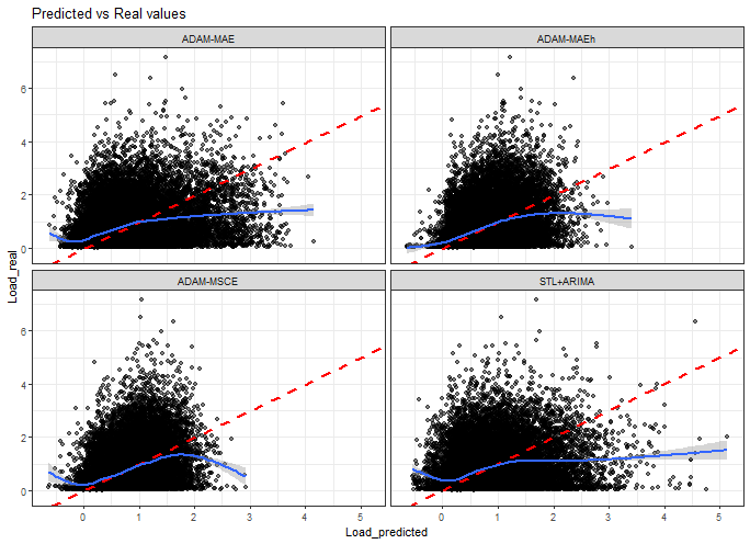

plot of chunk unnamed-chunk-15

That is not very nice behavior in general, actually :), there are a lot of below-zero predictions (but fewer with multistep losses!) and no high-load predictions with multistep losses.

Residuals vs real values scatter plot:

ggplot(data_predictions_all[model %in% models_sub],
       aes(Error, Load_real)) +
  facet_wrap(~model, scales = "fixed") +
  geom_point(alpha = 0.5) +
  geom_smooth(alpha = 0.6) +
  xlab("resid (predicted_value - Load_real)") +
  labs(title = "Residual vs Real values") +
  theme_bw()

## `geom_smooth()` using method = 'gam' and formula = 'y ~ s(x, bs = "cs")'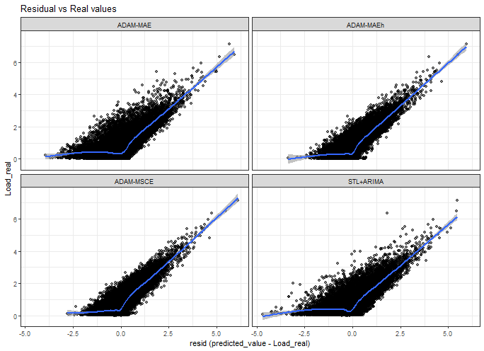

plot of chunk unnamed-chunk-16

Again, it is not a very nice plot :) the conclusions are very similar to with previous one.

Heteroscedasticity check - so real values vs. absolute errors.

ggplot(data_predictions_all[model %in% models_sub],
       aes(Load_real, AE)) +
  facet_wrap(~model, scales = "fixed") +
  geom_point(alpha = 0.5) +
  geom_smooth(alpha = 0.6) +
  ylab("abs(resid)") +
  labs(title = "heteroscedasticity check") + 
  theme_bw()

## `geom_smooth()` using method = 'gam' and formula = 'y ~ s(x, bs = "cs")'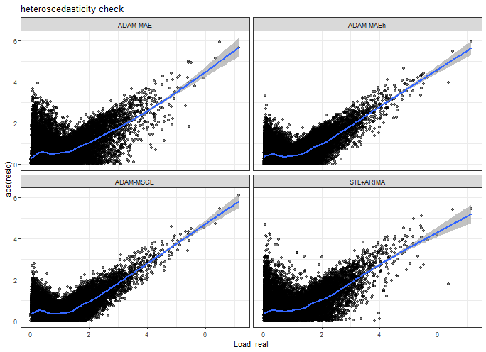

plot of chunk unnamed-chunk-17

Our models have no heteroscedasticity at all, so absolute errors are not similarly distributed around real values distribution.

Let’s see assumptions of normally distributed errors - Q-Q plot check:

ggplot(data_predictions_all[model %in% models_sub],
       aes(sample = Error, group = model)) +
  facet_wrap(~model, scales = "fixed") +
  stat_qq() + stat_qq_line() +
  ylab("resid (predicted_value - Load_real)") +
  theme_bw()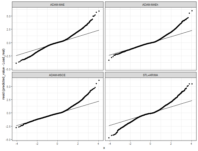

plot of chunk unnamed-chunk-18

We can see a nicer Q-Q plot with multistep losses - values are sliding on the optimal line much more than with benchmarks.

The last check is about the assumption that multistep forecasting errors have zero mean (will check it hourly - not by 15 minutes):

data_predictions_all[, Hour := lubridate::hour(Date_Time)]
 
ggplot(data_predictions_all[model %in% models_sub],
       aes(Hour, Error, group = Hour)) +
  facet_wrap(~model, scales = "free_y", ncol = 1) +
  geom_boxplot(alpha = 0.7, color = "black", fill = "gray") +
  geom_hline(yintercept = 0, color = "red") +
  geom_point(data = data_predictions_all[model %in% models_sub,
                                         .(Error = mean(Error)),
                                         by = .(model, Hour)],
             aes(Hour, Error, group = Hour), color = "firebrick2") +
  xlab("Hour (horizon)") +
  ylab("resid (predicted_value - Load_real)") +
  labs(title = "Multistep forecast errors have zero mean check") + 
  theme_bw()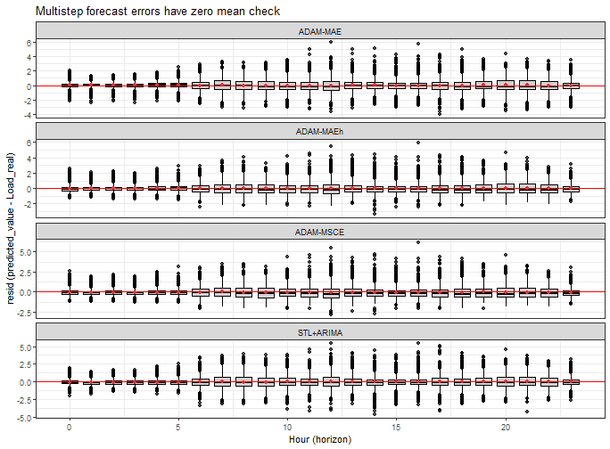

plot of chunk unnamed-chunk-19

All models are quite around zero, so good.

Summary

In this blog post, I showed that multistep losses in the ETS model have a great impact on forecast behavior:

lower variance,
and more accurate forecasts,

in our case of 1 day ahead household electricity consumption forecasting.

In general, household electricity consumption forecasting with ETS is not satisfactory as seen with model diagnostic methods that were showed -> higher values of consumption load are not well covered, etc.

In the future, I would like to show the possibility of improving forecasting accuracy with some ensemble methods, even with an ensemble of “weak” models such as ETS.

Seven coffees were consumed while writing this article.

If you’ve found it valuable, please consider supporting my work and...